Concept explainers
Videos
State the null and alternative hypothesis.
Find the degrees of freedom.
Find the critical value of chi-square from Appendix E or from Excel’s
Calculate the chi-square test statistics at 0.01 level of significance.
Interpret the p-value.
Check whether the conclusion is sensitive to the level of significance chosen, identify the cells that contribute to the chi-square test statistic and check for the small expected frequencies.
Draw histogram.
Test to obtain a probability plot with the Anderson-Darling statistic.
Interpret p-values.
Answer to Problem 40CE
The null hypothesis is:
And the alternative hypothesis is:
The degrees of freedom is 1.
The critical-value using EXCEL is 2.705543.
The chi-square test statistics at 0.1 level of significance is 0.0486.
The p-value for the hypothesis test is 0.825518.
There is enough evidence to conclude that the Circulated nickels come from a Normal population.
The conclusion is not sensitive to the level of significance chosen.
The chi-square test statistic has highest chi-square value for zero appointments.
There is no expected frequencies that are too small.
The histogram is:
The probability plot is:
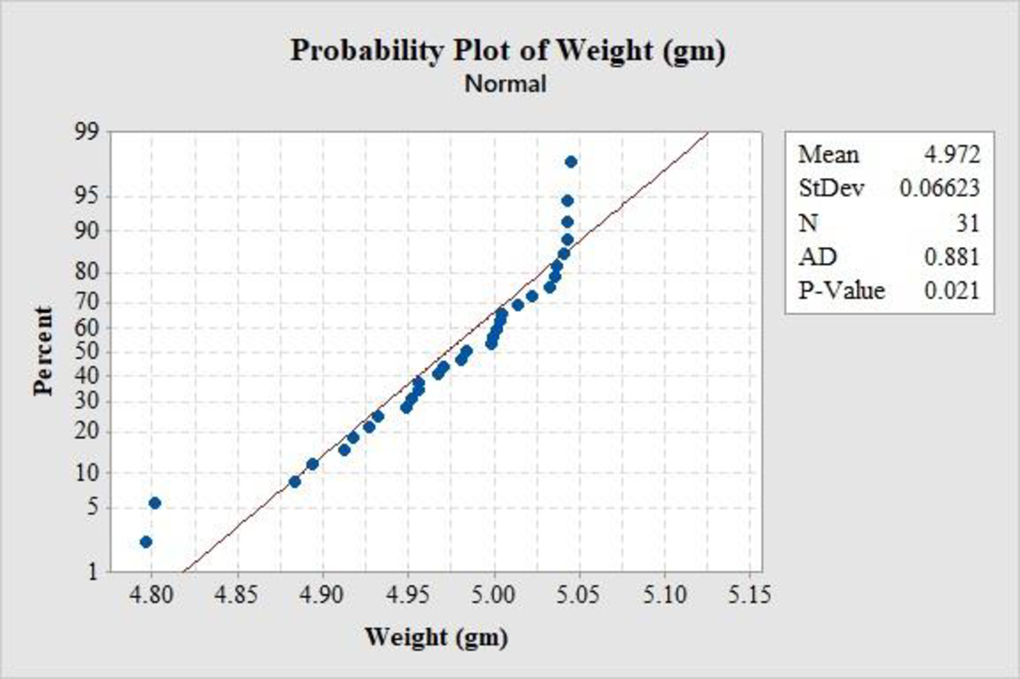
The Anderson-Darling statistics is 0.881.
The p-value is 0.021.
There is enough evidence to conclude that the Circulated nickels come from a Normal population.
Explanation of Solution
Calculation:
Results will vary.
The given information is the weights of 31 randomly chosen circulated nickels are given. There are 6 data set and pick any of them.
Here the data set F is considered
The claim is to test whether the data provide sufficient evidence to conclude that the Circulated nickels come from a Normal population. If the claim is rejected, then the Circulated nickels do not come from a Normal population.
The test hypotheses are given below:
Null hypothesis:
Alternative hypothesis:
Software procedure:
- Step by step procedure to obtain the mean and standard deviations using the MINITAB software is as follows,
- • Choose Stat > Basic Statistics>Display
Descriptive Statistics . - • Under Variables, choose 'Weight'
- • Choose Statistics, Select mean and Standard deviation.
- • Click OK.
Output obtained from MINITAB software for the data is:
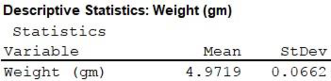
Thus, the mean and the standard deviation of the data is 4.9719 and 0.0662 respectively.
For a
Procedure for upper limit using EXCEL:
Step-by-step software procedure to obtain upper limit for first class using EXCEL is as follows:
- • Open an EXCEL file.
- • In cell A1, enter the formula “=NORM.INV(1/6,75.38,8.94)”
- Output using EXCEL software is given below:
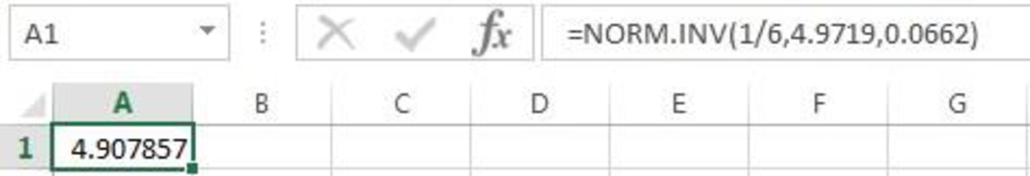
Thus, the upper limit for first class using EXCEL is 4.908.
Similarly the remaining limits can be obtained as shown below:
| Weights |
| Under 4.908 |
| 4.908–4.943 |
| 4.943–4.972 |
| 4.972–5.000 |
| 5.000–5.036 |
| 5.036 or more |
The expected frequency can be obtained by the following formula:
Where c is the number of bins and n is the sample size.
Substitute
Then the expected frequency for each bin can be obtained as shown in the table:
| Weights |
Expected Frequency |
| Under 4.908 | 5.17 |
| 4.908–4.943 | 5.17 |
| 4.943–4.972 | 5.17 |
| 4.972–5.000 | 5.17 |
| 5.000–5.036 | 5.17 |
| 5.036 or more | 5.17 |
| Total | 31 |
Frequency:
The frequencies are calculated by using the tally mark and the range of the data is from 4.796 to 5.045.
- • Based on the given information, the class intervals are under 4.908, 4.908–4.943, and so on, 5.036 or more.
- • Make a tally mark for each value in the corresponding class and continue for all values in the data.
- • The number of tally marks in each class represents the frequency, f of that class.
Similarly, the frequency of remaining classes for the emission is given below:
| Weights | Tally marks |
Observed Frequency |
| Under 4.908 | 4 | |
| 4.908–4.943 | 4 | |
| 4.943–4.972 | 6 | |
| 4.972–5.000 | 4 | |
| 5.000–5.036 | 8 | |
| 5.036 or more | 5 |
Let
The chi-square test statistics can be obtained by the formula:
Then the chi-square test statistics can be obtained as shown in the table:
| Weights |
Frequency |
Expected Frequency | ||
| Under 4.908 | 4 | 5.17 | –1.17 | 0.265 |
| 4.908–4.943 | 4 | 5.17 | –1.17 | 0.265 |
| 4.943–4.972 | 6 | 5.17 | 0.83 | 0.133 |
| 4.972–5.000 | 4 | 5.17 | –1.17 | 0.265 |
| 5.000–5.036 | 8 | 5.17 | 2.83 | 1.55 |
| 5.036 or more | 5 | 5.17 | –0.17 | 0.005 |
| Total | 31 | 31 | 0 | 2.483 |
Therefore, the chi-square test statistic is 2.483.
Degrees of freedom:
The degrees of freedom can be obtained as follows:
Where c is the number of classes and m is the number of parameters estimated. Here only 2 parameters are estimated.
Substitute 6 for c and 2 for m.
Thus, the degrees of freedom for the test is 3.
Procedure for p-value using EXCEL:
Step-by-step software procedure to obtain p-value using EXCEL software is as follows:
- • Open an EXCEL file.
- • In cell A1, enter the formula “=CHISQ.DIST.RT(2.483,3)”
- Output using EXCEL software is given below:
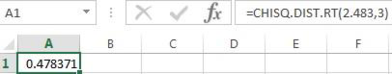
Thus, the p-value using EXCEL is 0.478.
Rejection rule:
If the p-value is less than or equal to the significance level, then reject the null hypothesis
Conclusion:
Here, the p-value is greater than the 0.01 level of significance.
That is,
Therefore, the null hypothesis is not rejected.
Thus, the data provide sufficient evidence to conclude that the Circulated nickels come from a Normal population.
Take
Here, the p-value is less than the 0.05 level of significance.
That is,
Therefore, the null hypothesis is not rejected.
Thus, the data provide sufficient evidence to conclude that the Circulated nickels come from a Normal population.
Thus, the conclusion is same for both the significance levels.
Hence, the conclusion is not sensitive to the level of significance chosen.
The class 5.000-5.036 contribute most to the chi-square test statistic.
Since all
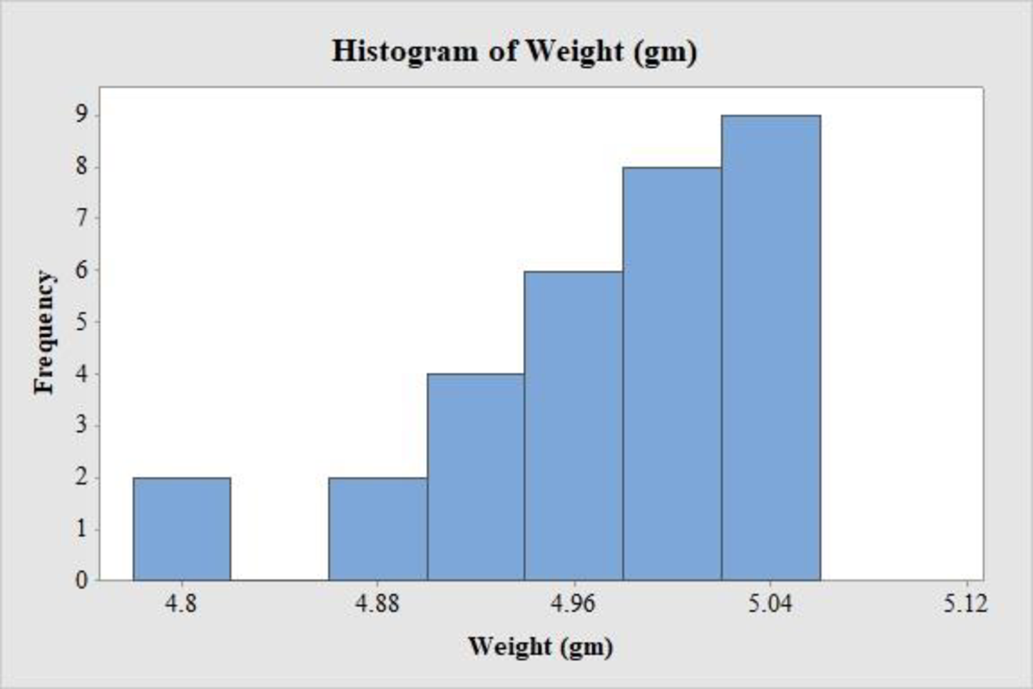
Frequency Histogram:
Software procedure:
- Step by step procedure to draw the relative frequency histogram for mileage for 2000 using MINITAB software is as follows,
- • Choose Graph > Histogram.
- • Choose Simple.
- • Click OK.
- • In Graph variables, enter the column of 'Weight'.
- • In Scale, Choose Y-scale Type as Frequency.
- • Click OK.
- • Select Edit Scale, Enter 4.8, 4.88, 4.96, 5.04, 5.12 in Positions of ticks.
- • In Labels, Enter 4.8, 4.88, 4.96, 5.04, 5.12 41 in Specified.
- • Click OK.
Observation:
It is clear that the histogram is not symmetric. The left hand tail is little longer than the right hand tail from the maximum frequency value. Thus, there is little negative skewness on the histogram.
Software procedure:
Step by step procedure to obtain the probability plot using the MINITAB software is as follows:
- • Choose Stat > Basic Statistics > Normality Test.
- • In Variable, enter the column of 'Weights'.
- • Under Test for Normality, select the column of Anderson-Darling.
- • Click OK.
From the probability plot, it can be observed that most of the observations lies near to the straight line. Therefore, the data is from a normal distribution.
From the MINITAB output the Anderson-Darling statistics is 0.881 and the p-value is 0.021.
Conclusion:
Here, the p-value is greater than the 0.01 level of significance.
That is,
Therefore, the null hypothesis is not rejected.
Thus, the data provide sufficient evidence to conclude that the Circulated nickels come from a Normal population.
Want to see more full solutions like this?
Chapter 15 Solutions
Loose-leaf For Applied Statistics In Business And Economics


 MATLAB: An Introduction with ApplicationsStatisticsISBN:9781119256830Author:Amos GilatPublisher:John Wiley & Sons Inc
 Probability and Statistics for Engineering and th...StatisticsISBN:9781305251809Author:Jay L. DevorePublisher:Cengage Learning
 Statistics for The Behavioral Sciences (MindTap C...StatisticsISBN:9781305504912Author:Frederick J Gravetter, Larry B. WallnauPublisher:Cengage Learning
 Elementary Statistics: Picturing the World (7th E...StatisticsISBN:9780134683416Author:Ron Larson, Betsy FarberPublisher:PEARSON
 The Basic Practice of StatisticsStatisticsISBN:9781319042578Author:David S. Moore, William I. Notz, Michael A. FlignerPublisher:W. H. Freeman
 Introduction to the Practice of StatisticsStatisticsISBN:9781319013387Author:David S. Moore, George P. McCabe, Bruce A. CraigPublisher:W. H. Freeman