
Concept explainers
Videos
a.
Construct the
Revise the control limits if needed.
a.
Answer to Problem 91SE
The
The revised control limits for
The trial control limits for
Explanation of Solution
Calculation:
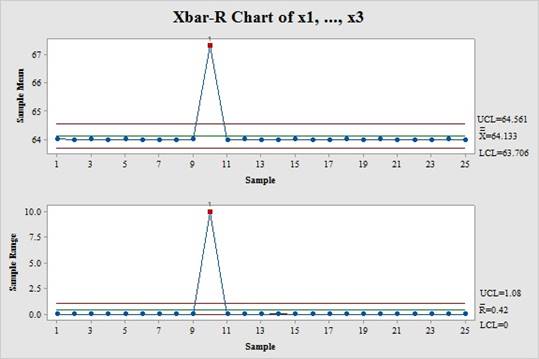
The data shows the diameter of fuse pins used in an aircraft engine taken for 25 samples and the sample subgroup size is 3.
Construction of
Software procedure:
Step-by-step procedure to construct
- Choose Stat > Control Charts > Variables Charts for Subgroups >Xbar-R.
- Choose Observations for a subgroup are in one row of columns and then enter columns of X1, X2 and X3.
- Click OK.
Interpretation:
The
Hence, the process is out of statistical control.
Revised control limits after eliminating the out of control data point:
Software procedure:
Step-by-step procedure to construct
- Choose Stat > Control Charts > Variables Charts for Subgroups >Xbar-R.
- Choose Observations for a subgroup are in one row of columns and then enter columns of X1, X2 and X3.
- Click OK.
Output obtained from MINITAB is given below:
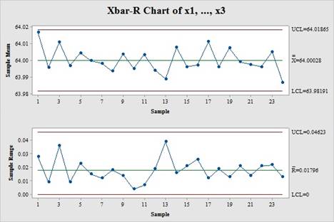
Interpretation:
The
Hence, the process is said to be in statistical control.
b.
Estimate the process mean and standard deviation.
b.
Answer to Problem 91SE
The estimate of the process mean is 64.
The estimate of the process standard deviation is 0.0106.
Explanation of Solution
Calculation:
From part (a) it can be observed that the
Process mean:
Thus, the estimate of the process mean is 64.
Process standard deviation:
Where,
The value of
- Locate the value of 3 under the column of
- Under the same row, locate the value for
Thus, the value of
Substitute 0.01796 as
Thus, the estimate of the process standard deviation is 0.0106.
c.
Calculate the estimate of PCR.
Identify whether the process meets the minimum capability level of
c.
Answer to Problem 91SE
The estimate of PCR is 0.63.
No, the process does not meet the minimum capability level of
Explanation of Solution
Calculation:
The given information is that the process specifications are stated at
The upper specification limit and lower specification limit are calculated as follows:
PCR:
Substitute USL as 64.02, LSL as 63.98 and
Thus, the value of PCR is 0.63.
Conclusion:
The process does not meet the minimum capability level of 1.33 since the estimate of PCR is 0.63 which is less than 1.33.
d.
Calculate the estimate of
Conclude about the process capability using the estimate of
d.
Answer to Problem 91SE
The estimate of
Explanation of Solution
Calculation:
Substitute USL as 64.02, LSL as 63.98,
Thus, the value of
Conclusion:
The process does not meet the minimum capability level of 1.33 since the estimate of
Hence, the process is not capable of operating within specification limits which is due to the values of PCR and
e.
Find the new value for the variance.
e.
Answer to Problem 91SE
The new value for the variance is 0.00001089.
Explanation of Solution
Calculation:
The given information is that to change this process as a 6 sigma process, the process variance should be decreased in such a way that the
Substitute LSL as 63.98,
Thus, the value of variance should be
f.
Find the probability that the shift is detected in the next sample.
Find the ARL value after the shift.
f.
Answer to Problem 91SE
The probability that the shift is detected in the next sample is 0.079.
The ARL value after the shift is 12.7.
Explanation of Solution
Calculation:
Assume that the process mean has shifted to 64.01
The probability of shift detected on the next sample is calculated by using the formula.
Where,
x represents the observed value of x.
The probability of shift detected on the next sample is calculated as follows:
Substitute 63.982 as LCL, 64.01865 as UCL, 64.01, 0.0106 as
Software procedure:
Step-by-step procedure to find the probability value using MINITAB is given below:
- Choose Graph > Probability Distribution Plot choose View Probability> OK.
- From Distribution, choose ‘Normal’ distribution.
- Click the Shaded Area tab.
- Choose X value and Middle Tail for the region of the curve to shade.
- Enter the X1 value as –4.59 and X2 value as 1.41.
- Click OK.
Output obtained from MINITAB is given below:
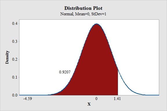
Thus, the probability of detecting a shift in the next sample is given below:
Hence, the probability of detecting a shift in the next sample is 0.079.
ARL:
It is the average run length of the control chart. ARL is the average number of data points which are plotted to indicate the out-of-control condition.
Where,
p represents the probability that a data points will exceed the control limits.
From part (b) it can be observed that the value of p is 0.079.
Thus, the ARL value is 12.7.
Conclusion:
Thus, the average run length after the shift is 12.7.
Want to see more full solutions like this?
Chapter 15 Solutions
Applied Statistics and Probability for Engineers 6e + WileyPLUS Registration Card


 MATLAB: An Introduction with ApplicationsStatisticsISBN:9781119256830Author:Amos GilatPublisher:John Wiley & Sons Inc
 Probability and Statistics for Engineering and th...StatisticsISBN:9781305251809Author:Jay L. DevorePublisher:Cengage Learning
 Statistics for The Behavioral Sciences (MindTap C...StatisticsISBN:9781305504912Author:Frederick J Gravetter, Larry B. WallnauPublisher:Cengage Learning
 Elementary Statistics: Picturing the World (7th E...StatisticsISBN:9780134683416Author:Ron Larson, Betsy FarberPublisher:PEARSON
 The Basic Practice of StatisticsStatisticsISBN:9781319042578Author:David S. Moore, William I. Notz, Michael A. FlignerPublisher:W. H. Freeman
 Introduction to the Practice of StatisticsStatisticsISBN:9781319013387Author:David S. Moore, George P. McCabe, Bruce A. CraigPublisher:W. H. Freeman