Introductory Statistics, Books a la Carte Plus NEW MyLab Statistics with Pearson eText -- Access Card Package (10th Edition)
10th Edition
ISBN: 9780134270364
Author: Neil A. Weiss
Publisher: PEARSON
expand_more
expand_more
format_list_bulleted
Videos
Textbook Question
Chapter 15.3, Problem 95E
In Exercises 15.92–15.9, presume that the assumptions for regression inferences are met.
15.95 Plaint Emissions. Following are the data on plant weight and quantity of volatile emissions from Exercise 15.25.
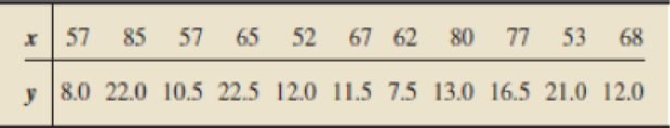
- a. Obtain a point estimate for the
mean quantity of volatile emissions of all (Solanum tuberosum) plants that weigh 60 g. - b. Find a 95% confidence interval for the mean quantity of volatile emissions of all plants that weigh 60 g.
- c. Find the predicted quantity of volatile emissions for a plant that weighs 60 g.
- d. Determine a 95% prediction interval for the quantity of volatile emissions for a plant that weighs 60 g.
Expert Solution & Answer
Want to see the full answer?
Check out a sample textbook solution
Students have asked these similar questions
The data in Table 7–6 were collected in a clinical trial to evaluate a new compound designed to improve wound healing in trauma patients. The new compound was com- pared against a placebo. After treatment for 5 days with the new compound or placebo, the extent of wound heal- ing was measured. Is there a difference in the extent of wound healing between the treatments? (Hint: Are treat- ment and the percent wound healing independent?) Run the appropriate test at a 5% level of significance. Can you please show how to do it in excel.
Treatment
0-25%
26-50%
51-75%
76-100%
New Compound (n=125)
15
37
32
41
Placebo
(n=125)
36
45
34
10
The table below lists measured amounts of redshift and the distances (billions of light-years) to randomly selected astronomical objects. There is sufficient evidence to support a claim of a linear correlation, so it is reasonable to use the regression equation when making predictions. For the prediction interval, use a 90% confidence level with a redshift of 0.0126. Find the explained variation.
A regression model to predict Y, the state burglary rate per 100,000 people, used the following four state predictors: X₁ = median age,
X₂ = number of bankruptcies per 1.000 population, X3 = federal expenditures per capita (a leading predictor), and X4 = high school
graduation percentage.
Click here for the Excel Data File
(a) Using the sample size of 50 people, calculate the calc and p-value in the table given below. (Negative values should be indicated
by a minus sign. Leave no cells blank - be certain to enter "0" wherever required. Round your answers to 4 decimal places.)
Predictor
Intercept
AgeMed
Bankrupt
FedSpend
HSGrad%
Answer is complete but not entirely correct.
*calc
5.2526
-2.1764✔✔
1.4101✔
Coefficient
4,198.5808
-27.3540
17.4893
-0.0124
-29.0314
SE
799.3395
12.5687
12.4033
0.0176
7.1268
-0.7045
-4.0736
p-value
0.0000
0.0348
0.2935
0.4848
0.0002
Chapter 15 Solutions
Introductory Statistics, Books a la Carte Plus NEW MyLab Statistics with Pearson eText -- Access Card Package (10th Edition)
Ch. 15.1 - Suppose that x and y are predictor and response...Ch. 15.1 - Prob. 2ECh. 15.1 - Prob. 3ECh. 15.1 - Prob. 4ECh. 15.1 - Prob. 5ECh. 15.1 - In Exercises 15.315.6, assume that the variables...Ch. 15.1 - The difference between an observed value and a...Ch. 15.1 - Identify two graphs used in a residual analysis to...Ch. 15.1 - Which graph used in a residual analysis provides...Ch. 15.1 - Figure 15.8 shows three residual plots and a...
Ch. 15.1 - Figure 15.9 on the next page shows three residual...Ch. 15.1 - In Exercises 15.1215.21, we repeat the data and...Ch. 15.1 - In Exercises 15.1215.21, we repeat the data and...Ch. 15.1 - Prob. 14ECh. 15.1 - Prob. 15ECh. 15.1 - Prob. 16ECh. 15.1 - Prob. 17ECh. 15.1 - Prob. 18ECh. 15.1 - Prob. 19ECh. 15.1 - Prob. 20ECh. 15.1 - Prob. 21ECh. 15.1 - Prob. 22ECh. 15.1 - Prob. 23ECh. 15.1 - Prob. 24ECh. 15.1 - Prob. 25ECh. 15.1 - In Exercises 15.2215.27, we repeat the information...Ch. 15.1 - Prob. 27ECh. 15.1 - Prob. 28ECh. 15.1 - In Exercises 15.2815.33, a. compute the standard...Ch. 15.1 - Prob. 30ECh. 15.1 - In Exercises 15.2815.33, a. compute the standard...Ch. 15.1 - In Exercises 15.2815.33, a. compute the standard...Ch. 15.1 - In Exercises 15.2815.33, a. compute the standard...Ch. 15.1 - In Exercises 15.3415.43, use the technology of...Ch. 15.1 - In Exercises 15.3415.43, use the technology of...Ch. 15.1 - In Exercises 15.3415.43, use the technology of...Ch. 15.1 - In Exercises 15.3415.43, use the technology of...Ch. 15.1 - Prob. 38ECh. 15.1 - Prob. 39ECh. 15.1 - Prob. 40ECh. 15.1 - Prob. 41ECh. 15.1 - Prob. 42ECh. 15.1 - Prob. 43ECh. 15.2 - Explain why the predictor variable is useless as a...Ch. 15.2 - Prob. 45ECh. 15.2 - Prob. 46ECh. 15.2 - In this section, we used the statistic b1 as a...Ch. 15.2 - In Exercises 15.4815.57, we repeat the information...Ch. 15.2 - Prob. 49ECh. 15.2 - In Exercises 15.4815.57, we repeat the information...Ch. 15.2 - In Exercises 15.4815.57, we repeat the information...Ch. 15.2 - Prob. 52ECh. 15.2 - Prob. 53ECh. 15.2 - Prob. 54ECh. 15.2 - In Exercises 15.4815.57, we repeat the information...Ch. 15.2 - Prob. 56ECh. 15.2 - Prob. 57ECh. 15.2 - Prob. 58ECh. 15.2 - In Exercises 15.5815.63, we repeat the information...Ch. 15.2 - Prob. 60ECh. 15.2 - In Exercises 15.5815.63, we repeat the information...Ch. 15.2 - Prob. 62ECh. 15.2 - In Exercises 15.5815.63, we repeat the information...Ch. 15.2 - Prob. 64ECh. 15.2 - In each of Exercises 15.6415.69, apply Procedure...Ch. 15.2 - In each of Exercises 15.6415.69, apply Procedure...Ch. 15.2 - Prob. 67ECh. 15.2 - Prob. 68ECh. 15.2 - Prob. 69ECh. 15.2 - Prob. 70ECh. 15.2 - In Exercises 15.7015.80, use the technology of...Ch. 15.2 - In Exercises 15.7015.80, use the technology of...Ch. 15.2 - Prob. 73ECh. 15.2 - Prob. 74ECh. 15.2 - Prob. 75ECh. 15.2 - In Exercises 15.7015.80, use the technology of...Ch. 15.2 - Prob. 77ECh. 15.2 - Prob. 78ECh. 15.2 - In Exercises 15.7015.80, use the technology of...Ch. 15.2 - Prob. 80ECh. 15.3 - Without doing any calculations, fill in the blank....Ch. 15.3 - Prob. 82ECh. 15.3 - Prob. 83ECh. 15.3 - Prob. 84ECh. 15.3 - In Exercises 15.8215.91, we repeat the data from...Ch. 15.3 - Prob. 86ECh. 15.3 - Prob. 87ECh. 15.3 - In Exercises 15.8215.91, we repeat the data from...Ch. 15.3 - Prob. 89ECh. 15.3 - Prob. 90ECh. 15.3 - Prob. 91ECh. 15.3 - Prob. 92ECh. 15.3 - In Exercises 15.9215.97, presume that the...Ch. 15.3 - In Exercises 15.9215.97, presume that the...Ch. 15.3 - In Exercises 15.9215.9, presume that the...Ch. 15.3 - Prob. 96ECh. 15.3 - In Exercises 15.9215.97, presume that the...Ch. 15.3 - Prob. 98ECh. 15.3 - In Exercises 15.9815.108, use the technology of...Ch. 15.3 - In Exercises 15.9815.108, use the technology of...Ch. 15.3 - In Exercises 15.9815.108, use the technology of...Ch. 15.3 - In Exercises 15.9815.108, use the technology of...Ch. 15.3 - Prob. 103ECh. 15.3 - Prob. 104ECh. 15.3 - Prob. 105ECh. 15.3 - Prob. 106ECh. 15.3 - In Exercises 15.9815.108, use the technology of...Ch. 15.3 - Prob. 108ECh. 15.3 - Margin of Error in Regression. In Exercises 15.109...Ch. 15.3 - Refer to the confidence interval and prediction...Ch. 15.4 - Identify the statistic used to estimate the...Ch. 15.4 - Prob. 112ECh. 15.4 - Suppose that, for a sample of pairs of...Ch. 15.4 - Prob. 114ECh. 15.4 - Prob. 115ECh. 15.4 - Prob. 116ECh. 15.4 - Prob. 117ECh. 15.4 - Prob. 118ECh. 15.4 - Prob. 119ECh. 15.4 - Prob. 120ECh. 15.4 - Prob. 121ECh. 15.4 - Prob. 122ECh. 15.4 - Prob. 123ECh. 15.4 - Prob. 124ECh. 15.4 - Prob. 125ECh. 15.4 - Prob. 126ECh. 15.4 - Prob. 127ECh. 15.4 - Prob. 128ECh. 15.4 - Prob. 129ECh. 15.4 - Prob. 130ECh. 15.4 - Prob. 131ECh. 15.4 - Prob. 132ECh. 15.4 - Prob. 133ECh. 15.4 - In each of Exercises 15.13415.144, use the...Ch. 15.4 - In each of Exercises 15.13415.144, use the...Ch. 15.4 - Prob. 136ECh. 15.4 - Prob. 137ECh. 15.4 - Prob. 138ECh. 15.4 - Prob. 139ECh. 15.4 - Prob. 140ECh. 15.4 - In each of Exercises 15.13415.144, use the...Ch. 15.4 - Prob. 142ECh. 15.4 - Prob. 143ECh. 15.4 - Prob. 144ECh. 15 - Prob. 1RPCh. 15 - Suppose that x and y are two variables of a...Ch. 15 - What two plots did we use in this chapter to...Ch. 15 - Regarding analysis of residuals, decide in each...Ch. 15 - Suppose that you perform a hypothesis test for the...Ch. 15 - Prob. 6RPCh. 15 - Prob. 7RPCh. 15 - Prob. 8RPCh. 15 - Prob. 9RPCh. 15 - Identify the relationship between two variables...Ch. 15 - Graduation Rates. Graduation ratethe percentage of...Ch. 15 - Prob. 12RPCh. 15 - Prob. 13RPCh. 15 - For Problems 1417, presume that the variables...Ch. 15 - For Problems 1417, presume that the variables...Ch. 15 - For Problems 1417, presume that the variables...Ch. 15 - Prob. 17RPCh. 15 - In Problems 1820, use the technology of your...Ch. 15 - In Problems 1820, use the technology of your...Ch. 15 - In Problems 1820, use the technology of your...Ch. 15 - Recall from Chapter 1 (see page 34) that the Focus...Ch. 15 - At the beginning of this chapter, we presented...
Knowledge Booster


Learn more about
Need a deep-dive on the concept behind this application? Look no further. Learn more about this topic, statistics and related others by exploring similar questions and additional content below.Similar questions
- To perform a test to determine whether we have a significant linear relationship using an F test, your friend tells you to compute a two-sided p-value. Is this correct and why?arrow_forwardStephen Stigler determined in 1977 that the speed of light is 299,710.5 km/sec. In 1882, Albert Michelson had collected measurements on the speed of light ("Student t-distribution," 2013). His measurements are given in table #7.3.6. Is there evidence to show that Michelson’s data is different from Stigler’s value of the speed of light? Test at the 5% level. Table #7.3.6: Speed of Light Measurements in (km/sec) 299883 299816 299778 299796 299682 299711 299611 299599 300051 299781 299578 299796 299774 299820 299772 299696 299573 299748 299748 299797 299851 299809 299723arrow_forwardan attempt to develop a model of wine quality as judged by wine experts, data on alcohol content and wine quality was collected from variants of a particular wine. From a sample of 12wines, a model was created using the percentages of alcohol to predict wine quality. For those data, SR=18,671 and SST=27,382.Use this information to complete parts (a) through (c) below. Please complete part 3(B) ONLY. Question content area bottom Part 1 a. Determine the coefficient of determination, r2, and interpret its meaning. r2=0.682 (Round to three decimal places as needed.) Part 2 Interpret the meaning of r2. It means that 68.2 of the variation in wine quality can be explained by the variation in alcohol content. (Round to one decimal place as needed.) Part 3 b. Determine the standard error of the estimate. SYX= (Round to four decimal places as needed.)arrow_forward
- Report the correlations between the three independent variables (age, educ and Protestant) and your dependent variable (childs). Which category had the correlation that was the weakest?arrow_forwardA methodological study had established values for the MIC on a scale that measured physical function: The MIC for improvement (higher scores) was 4.0, and the MIC for deterioration (lower scores) was 3.0. Lawrence studied clinically significant change in physical functioning over a 1-year period for a sample of 100 patients with COPD. Some change score information is presented below for 10 patients. Which patients experienced clinically significant change in physical function in the 12-month period between assessments? Patient Baseline Score* 12-Month Score* 1 19 15 2 12 10 3 16 14 4 17 16 5 9 10 6 11 12 7 13 17 8 15 13 9 18 14 10 16 9 *Higher scores = higher level of physical function Which patients had clinically significant deterioration? Which patients had clinically significant improvement? Which patients had no clinically significant change?arrow_forwardFor a given set of x and y data values, assume that the regression model assumptions are valid and that a 90% confidence interval for ₁ is given by (-2.2, -0.1). Which of the following statements are true? i) At a = 0.10, there is a significant linear relationship between x and y. ii) In the scatterplot of x and y, the values of y tend to decrease as the values of x increase. iii) Based on this confidence interval, we would reject the null hypothesis of no linear relationship at any significance level a ≤ 0.1. Select one: a. i) O b. i) and ii) O c. ii) d. i), ii), and iii)arrow_forward
- The table below lists measured amounts of redshift and the distances (billions of light-years) to randomly selected astronomical objects. Find the (a) explained variation, (b) unexplained variation, and (c) indicated prediction interval. There is sufficient evidence to support a claim of a linear correlation, so it is reasonable to use the regression equation when making predictions. For the prediction interval, use a 90% confidence leve with a redshift of 0.0126. Redshift Distance 0.0231 0.31 a. Find the explained variation. 0.0536 0.77 (Round to six decimal places as needed.) b. Find the unexplained variation. (Round to six decimal places as needed.) c. Find the indicated prediction interval. 0.0716 0.0395 1.01 0.53 billion light-yearsarrow_forwardAn experiment was conducted to evaluate the effect of decreases in frontalis muscle tension on headaches. The number of headaches experienced in a 2-week baseline period was recorded in 9 subjects who had been experiencing tension headaches. Then the subjects were trained to lower frontalis muscle tension using biofeedback, after which the number of headaches in another 2-week period was again recorded. The data are shown below. No. of Headaches Subject No Baseline After Training 1 17 3 2 13 7 3 6 2 4 5 3 5 5 6 6 10 2 7 8 1 8 6 0 9 7 2 Assume the t-test cannot be used because of an extreme violation of its normality assumption. Use the Wilcoxon signed ranks test to analyze the data. What do you conclude, using α = 0.05 2tail?arrow_forward20arrow_forwardA regression model to predict Y, the state burglary rate per 100,000 people, used the following four state predictors: X₁ = median age, X₂ = number of bankruptcies per 1,000 population, X3 = federal expenditures per capita (a leading predictor), and X4 = high school graduation percentage. Click here for the Excel Data File (a) Using the sample size of 50 people, calculate the tcalc and p-value in the table given below. (Negative values should be indicated by a minus sign. Leave no cells blank - be certain to enter "0" wherever required. Round your answers to 4 decimal places.) Predictor Intercept AgeMed Bankrupt FedSpend HSGrad% Coefficient t-value = 4,198.5808 -27.3540 17.4893 -0.0124 -29.0314 SE 799.3395 12.5687 12.4033 0.0176 7.1268 tcalc p-value (b-1) What is the critical value of Student's t in Appendix D for a two-tailed test at a = .01? (Round your answer to 3 decimal places.)arrow_forwardThe fish in my pond have mean lenth 14 inches with a standard deviation of 2 inches and mean weight 4 pounds with a standard deviation of .8 pounds. The correlation coefficient of length and weight is .4. If the length of a particular randomly selected fish is reported to be 15 inches, then what should we predict for the weight of that fish using simple linear regression?arrow_forwardВ. A model estimated using a dataset with 125 observations generates the following results. SS df MS Regression 919587.543 4 229896.9 Error 2590390.62 121 534.2113 Std. Variable B Error t P>lt| X2 -0.0126355 0.005519 -2.28937 0.022 X3 0.5957923 0.014482 41.13934 0.000 Х4 1.124589 0.877192 1.282032 0.200 X5 0.3237421 0.060709 5.332661 0.000 constant 8.86016 1.766116 5.016749 0.000 What is the R2 for this sample? What information does the R² provide?arrow_forwardarrow_back_iosSEE MORE QUESTIONSarrow_forward_ios
Recommended textbooks for you
 Glencoe Algebra 1, Student Edition, 9780079039897...AlgebraISBN:9780079039897Author:CarterPublisher:McGraw Hill
 Big Ideas Math A Bridge To Success Algebra 1: Stu...AlgebraISBN:9781680331141Author:HOUGHTON MIFFLIN HARCOURTPublisher:Houghton Mifflin Harcourt
Glencoe Algebra 1, Student Edition, 9780079039897...
Algebra
ISBN:9780079039897
Author:Carter
Publisher:McGraw Hill
Big Ideas Math A Bridge To Success Algebra 1: Stu...
Algebra
ISBN:9781680331141
Author:HOUGHTON MIFFLIN HARCOURT
Publisher:Houghton Mifflin Harcourt
Hypothesis Testing using Confidence Interval Approach; Author: BUM2413 Applied Statistics UMP;https://www.youtube.com/watch?v=Hq1l3e9pLyY;License: Standard YouTube License, CC-BY
Hypothesis Testing - Difference of Two Means - Student's -Distribution & Normal Distribution; Author: The Organic Chemistry Tutor;https://www.youtube.com/watch?v=UcZwyzwWU7o;License: Standard Youtube License