
STATISTICSMYSTAT LAB ACCESS CODE + PHS
13th Edition
ISBN: 9780134613949
Author: MCCLAVE
Publisher: PEARSON
expand_more
expand_more
format_list_bulleted
Concept explainers
Videos
Textbook Question
Chapter 15.7, Problem 15.70ACB
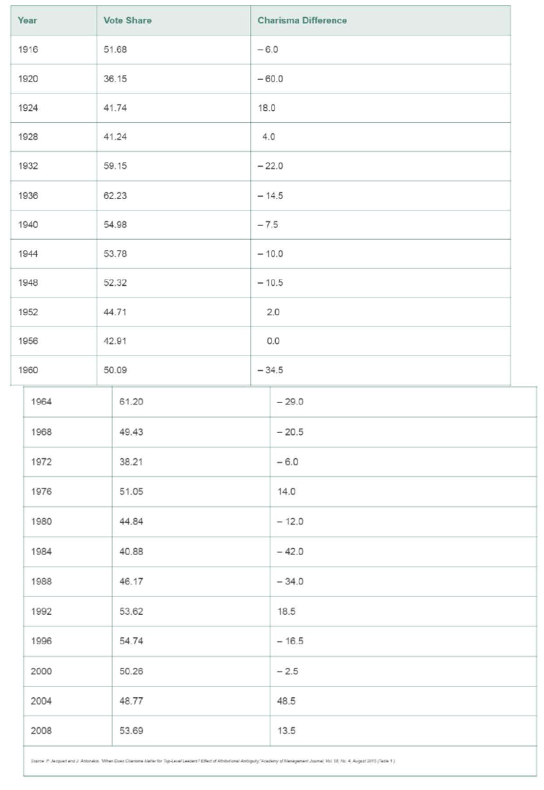
Charisma of top-level leaders. Refer to the Academy of Management Journal (August 2015) study of the charisma of top business leaders, Exercise 11.28 (p. 633). Recall that researchers collected data on 24 U.S. presidential elections from 1916 to 2008. Two variables of interest were Democratic vote share (measured as the percentage of voters who voted for the Democratic candidate in the national election) and the difference between the Democratic and Republican candidates' charisma values (both measured on a 150-point scale). These data are reproduced in the accompanying table.
- a. Rank the Democratic vote share values.
- b. Rank the charisma difference values.
- c. Compute the differences in the ranks, part b.
- d. Use the results, part c, to find Spearman’s rank
correlation coefficient between Democratic vote share and charisma difference.
Expert Solution & Answer
Want to see the full answer?
Check out a sample textbook solution
Students have asked these similar questions
A U.S. study published in The American Journal of Preventive Medicine compared state-level prevalence of firearm ownership in 2002 with state-level rates of firearm assault and firearm robbery in the subsequent year. The investigators found a positive association - meaning that states with higher prevalence of firearm ownership also tended to be the states with higher rates of firearm assault.
Which design best describes this study?
a)Observational cohort study
b)Randomized trial
c)Case-control study
d)Ecological study
Does posting calorie content for menu items affectpeople’s choices in fast-food restaurants? According to results obtained by Elbel, Gyamfi, and Kersh(2011), the answer is no. The researchers monitoredthe calorie content of food purchases for children andadolescents in four large fast-food chains before andafter mandatory labeling began in New York City. Although most of the adolescents reported noticing thecalorie labels, apparently the labels had no effect ontheir choices. Data similar to the results obtained showan average of M = 786 calories per meal with s =85 for n =100 children and adolescents before thelabeling, compared to an average of M = 772 calorieswith s = 91 for a similar sample of n = 100 after themandatory posting.a. Use a two-tailed test with a = .05 to determinewhether the mean number of calories after theposting is significantly different than before caloriecontent was posted.b. Calculate r2to measure effect size for the mean difference.
The director of an obesity clinic in a large northwestern city believes that drinking soft drinks contribute to obesity in children. To determine whether a relationship exists between these two variables, she conducts the following pilot study. Eight- 12-year-old male volunteers are randomly selected from children attending a local junior high school. Parents of the children are asked to monitor the number of soft drinks consumed by their child over a one week period. The children are weighed at the end of the week and their weights converted into body mass index (BMI) values. The BMI is a common index used to measure obesity and takes into account both height and weight. An individual is considered obese if they have a BMI value 30. The following data or collected:
child. # of soft drinks consumed BMI
1 3 20
2 1 18
3…
Chapter 15 Solutions
STATISTICSMYSTAT LAB ACCESS CODE + PHS
Ch. 15.2 - Under what circumstances is the sign test...Ch. 15.2 - What is the probability that a randomly selected...Ch. 15.2 - Use Table I of Appendix D to calculate the...Ch. 15.2 - Consider the following sample of 10 measurements....Ch. 15.2 - Suppose you wish to conduct a test of the research...Ch. 15.2 - Accidents at construction sites. Refer to the...Ch. 15.2 - Salaries of experienced MBA graduates. According...Ch. 15.2 - Caffeine in Starbucks coffee. Researchers at the...Ch. 15.2 - Short-sale stock returns. The Securities and...Ch. 15.2 - Lobster trap placement. Refer to the Bulletin of...
Ch. 15.2 - Repair and replacement costs of water pipes. Refer...Ch. 15.2 - Performance of stock screeners. Refer to Exercise...Ch. 15.2 - Radon exposure in Egyptian tombs. Refer to the...Ch. 15.2 - Prob. 15.14ACICh. 15.3 - Prob. 15.15LMCh. 15.3 - Specify the test statistic and the rejection...Ch. 15.3 - Prob. 15.17LMCh. 15.3 - Prob. 15.18LMCh. 15.3 - Prob. 15.19ACBCh. 15.3 - Prob. 15.21ACBCh. 15.3 - Prob. 15.22ACBCh. 15.3 - The X-Factor in golf performance. Many golf...Ch. 15.3 - Prob. 15.24ACICh. 15.3 - Prob. 15.25ACICh. 15.3 - Prob. 15.26ACICh. 15.3 - Does rudeness really matter in the workplace?...Ch. 15.3 - Prob. 15.28ACICh. 15.4 - Prob. 15.29LMCh. 15.4 - Prob. 15.30LMCh. 15.4 - Prob. 15.31LMCh. 15.4 - Prob. 15.32LMCh. 15.4 - Twinned drill holes. Refer to the Exploration and...Ch. 15.4 - Prob. 15.34ACBCh. 15.4 - Prob. 15.35ACBCh. 15.4 - Prob. 15.36ACBCh. 15.4 - Prob. 15.37ACBCh. 15.4 - Prob. 15.38ACICh. 15.4 - Prob. 15.39ACICh. 15.4 - Prob. 15.40ACICh. 15.4 - Prob. 15.41ACICh. 15.4 - Prob. 15.42ACICh. 15.5 - Under what circumstances does the 2 distribution...Ch. 15.5 - Data were collected from three populations, A, B....Ch. 15.5 - Prob. 15.45LMCh. 15.5 - Prob. 15.46ACBCh. 15.5 - Prob. 15.47ACBCh. 15.5 - Prob. 15.48ACBCh. 15.5 - Prob. 15.49ACBCh. 15.5 - Prob. 15.50ACICh. 15.5 - Public defenders salaries. Random samples of seven...Ch. 15.5 - Prob. 15.52ACICh. 15.5 - Prob. 15.53ACICh. 15.6 - Prob. 15.54LMCh. 15.6 - Prob. 15.55LMCh. 15.6 - Prob. 15.56LMCh. 15.6 - Prob. 15.57ACBCh. 15.6 - Condit ions impeding farm production. A review of...Ch. 15.6 - Peer mentor training at a firm. Refer to the...Ch. 15.6 - Prob. 15.60ACBCh. 15.6 - Prob. 15.61ACICh. 15.6 - Prob. 15.62ACICh. 15.6 - Prob. 15.63ACICh. 15.6 - Prob. 15.64ACICh. 15.6 - Prob. 15.65ACICh. 15.7 - Prob. 15.66LMCh. 15.7 - Prob. 15.67LMCh. 15.7 - The following sample data were collected on...Ch. 15.7 - Compute Spearman s rank correlation coefficient...Ch. 15.7 - Charisma of top-level leaders. Refer to the...Ch. 15.7 - Prob. 15.71ACBCh. 15.7 - Prob. 15.72ACBCh. 15.7 - Prob. 15.73ACBCh. 15.7 - Prob. 15.74ACICh. 15.7 - Prob. 15.75ACICh. 15.7 - Prob. 15.76ACICh. 15.7 - Prob. 15.77ACICh. 15.7 - Sweetness of orange juice Refer to the orange...Ch. 15.7 - Americas most reputable companies. Forbes magazine...Ch. 15 - The data for three independent random samples are...Ch. 15 - Prob. 15.81LMCh. 15 - Two independent random samples produced the...Ch. 15 - Prob. 15.83LMCh. 15 - Prob. 15.84ACBCh. 15 - Prob. 15.85ACBCh. 15 - Office rental growth rates Real estate market...Ch. 15 - RIF plan to fire older employees. Reducing the...Ch. 15 - Prob. 15.88ACBCh. 15 - Wine-tasting experiment. Two expert wine tasters...Ch. 15 - Employee suggestion system. An employee suggestion...Ch. 15 - Prob. 15.91ACICh. 15 - Prob. 15.92ACICh. 15 - Prob. 15.93ACICh. 15 - Prob. 15.94ACICh. 15 - Cooling method for gas turbines. Refer to the...Ch. 15 - Flexible working hours program. A job-scheduling...Ch. 15 - Fluoride in drinking water. Many water treatment...Ch. 15 - Does fatigue lead to more defectives? A...Ch. 15 - Prob. 15.99ACICh. 15 - Prob. 15.100ACICh. 15 - Prob. 15.101ACICh. 15 - Groundwater contamination of wells. Methyl...
Knowledge Booster


Learn more about
Need a deep-dive on the concept behind this application? Look no further. Learn more about this topic, statistics and related others by exploring similar questions and additional content below.Similar questions
- Which of the independent variables retains the strongest association with the number of children a respondent has when all other variables in the model are controlled? What is that association? Which has the weakest when other variables are controlled?arrow_forwardIn a study conducted in the Science Department of Faculty of Science, Technology and Human Development in a University; the researcher examined the influence of the drug succinylcholine on the circulation levels of androgens in the blood. Blood samples from wild, free-ranging deer were obtained via the jugular vein immediately after an intramuscular injection of succinylcholine using darts and a capture gun. Deer were bled again approximately 30 minutes after the injection and then released. The level of androgens at time of capture and 30 minutes later, measured in nanograms per milliliter (ng/ml), for 15 deers as in Table Q1. Assuming that the populations of androgen at time of injection and 30 minutes later are normally distributed:i) Find the average and standard deviation of this studyii)Determine the critical region of this problem.iii) Test at the 0.05 level of significance whether the androgen concentrations are altered after 30 minutes of restraint.arrow_forwardIn the empirical exercises on earning and height in Chapters 4 and 5, you estimated a relatively large and statistically significant effect of a worker’s height on his or her earnings. One explanation for this result is omitted variable bias: Height is correlated with an omitted factor that affects earnings. For example, Case and Paxson (2008) suggest that cognitive ability (or intelligence) is the omitted factor. The mechanism they describe is straightforward: Poor nutrition and other harmful environmental factors in utero and in early childhood have, on average, deleterious effects on both cognitive and physical development. Cognitive ability affects earnings later in life and thus is an omitted variable in the regression. Suppose that the mechanism described above is correct. Explain how this leads to omitted variable bias in the OLS regression of Earnings on Height. Does the bias lead the estimated slope to be too large or too small? [Hint: Review Equation (6.1)]arrow_forward
- McAllister et al. (2012) compared varsity football and hockey players with varsity athletes from non-contact sports to determine whether exposure to head impacts during one season have an effect on cognitive performance. In the study, tests of new learning performance were significantly poorer for the contact sport athletes compared to the non-contact sport athletes. Cognitive Performance Contact Athletes Non-Contact Athletes n1 = 8 n2 = 8 M1 = 6 M2 = 9 s2 = 8 s2 = 6.23 Are the test scores significantly lower for the contact sport athletes than for the non-contact athletes? Conduct the appropriate hypothesis test using α = .05 and state your conclusion in terms of this problem. Make sure to use APA style conclusions (as shown in lecture videos).arrow_forwardintroduces a study investigating whether a brief diet intervention might improve depression symptoms. In the study, 75 college-age students with elevated depression symptoms and relatively poor diet habits were randomly assigned to either a healthy diet group or a control group. Depression levels were measured at the beginning of the experiment and then again three weeks later. The response variable is the reduction in depression level (as measured by the DASS survey) at the end of the three weeks. Larger numbers mean more improvement in depression symptoms. Test whether these experimental results allow us to conclude that, on average, improvement of depression symptoms is higher for those who eat a healthy diet for three weeks than for those who don't. The data is available on StatKey and in DietDepression. Let Group 1 represent those with a healthy diet and Group 2 represent those with no diet change. State the null and alternative hypotheses.arrow_forwardDowns and Abwender (2002) evaluated soccer players and swimmers to determine whether the routine blows to the head experienced by soccer players produced long term neurological deficits. In the study, neurological tests were administered to mature soccer players and swimmers and the results indicated significant differences. In a similar study, a researcher obtained the following data. Swimmers Soccer Players 10 7 8 4 7 9 9 3 13 7 7 6 12 a)Are the neurological test scores significantly lower for the soccer player than for the swimmers in the control groups? Use a one-tailed test with = .05. b)Compute the value of r² (percentage of variance accounted for) these data.arrow_forward
- In studies examining the effect of humor on interpersonal attractions, McGee and Shevlin (2009) found that an individual’s sense of humor had a significant effect on how the individual was perceived by others. In one part of the study, female college students were given brief descriptions of a potential romantic partner. The fictitious male was described positively as being single and ambitious and having good job prospects. For one group of participants, the description also said that he had a great sense of humor. For another group, it said that he has no sense of humor. After reading the description, each participant was asked to rate the attractiveness of the man on a seven-point scale from 1 (very unattractive) to 7 (very attractive). A score of 4 indicates a neutral rating. The females who read the “great sense of humor” description gave the potential partner an average attractiveness score of M = 4.53 with a standard deviation of s = 1.04. If the sample consisted of n = 16…arrow_forwardKnight and Haslam (2010) found that office workers who had some input into the design of their office space were more productive and had higher well-being compared to workers for whom the office design was completely controlled by an office manager. For this study, identify the independent variable and the dependent variablearrow_forwardLeisure Activities and Dementia. An article appearing in the Los Angeles Times discussed the study “Leisure Activities and the Risk of Dementia in the Elderly” (New England Journal of Medicine, Vol. 348) by J.Verghese et al. The article in the Times, titled “Crosswords Reduce Risk of Dementia,” contained the following statement: “Elderly people who frequently read, do crossword puzzles, practice a musical instrument or play board games cut their risk of Alzheimer’s and other forms of dementia by nearly two-thirds compared with people who seldom do such activities.” Comment on thestatement in quotes, keeping in mind the type of study for which causation can be reasonably inferred.arrow_forward
- A cross-sectional study is conducted to investigate cardiovascular disease (CVD) risk factors among a sample of patients seeking medical care at one of three local hospitals. A total of 500500 patients are enrolled. Based on the following data, we would like to determine if there is a significant association between the family history of CVD and the enrollment site. Enrollment Site Family History of CVD Hospital 1 Hospital 2 Hospital 3 Total Yes 34 8 58 100 No 104 72 224 400 Total 138 80 282 500 Given: The value of the test statistic is χ2= 6.912 Use α=0.1 as the level of significance. The superintendent of Hospital 2 performed the Goodness of Fit Test to test whether 25% of the patients go to Hospital 1, 15% of the patients go to Hospital 2 and 60% of the patients go to Hospital 3. Given: The superintendent found that the pp-value for the test is 0.25091 Let: p1=p1= be the proportion of patients at Hospital 1 p2=p2= be the proportion of patients at…arrow_forwardIn the book Business Research Methods (5th ed.), Donald R. Cooper and C. William Emory discuss studying the relationship between on-the-job accidents and smoking. Cooper and Emory describe the study as follows: Suppose a manager implementing a smoke-free workplace policy is interested in whether smoking affects worker accidents. Since the company has complete reports of on-the-job accidents, she draws a sample of names of workers who were involved in accidents during the last year. A similar sample from among workers who had no reported accidents in the last year is drawn. She interviews members of both groups to determine if they are smokers or not. The sample results are given in the following table. On-the-Job Accident Smoker Yes No Row Total Heavy 12 5 17 Moderate 9 10 19 Nonsmoker 13 17 30 Column total 34 32 66 Expected counts are below observed counts Accident No Accident Total Heavy 12 5 17 8.76 8.24…arrow_forwardA small random sample of respondents has been selected for a study of the ways that iPhone owners use their apps. Specifically, a research firm is comparing the apps for Starbucks, Amazon.com, and Yelp. Are there statistically significant differences by app for any of the variables listed here? Percent of battery used by the app in the last 24 hours Starbucks App Amazon App Yelp App 5 6 5 7 8 5 8 11 11 11 12 10 8 12 9 9 11 6 8 11 10 3 9 7 9 10 9 10 12 8arrow_forward
arrow_back_ios
SEE MORE QUESTIONS
arrow_forward_ios
Recommended textbooks for you
 Glencoe Algebra 1, Student Edition, 9780079039897...AlgebraISBN:9780079039897Author:CarterPublisher:McGraw Hill
 Big Ideas Math A Bridge To Success Algebra 1: Stu...AlgebraISBN:9781680331141Author:HOUGHTON MIFFLIN HARCOURTPublisher:Houghton Mifflin Harcourt
Glencoe Algebra 1, Student Edition, 9780079039897...
Algebra
ISBN:9780079039897
Author:Carter
Publisher:McGraw Hill
Big Ideas Math A Bridge To Success Algebra 1: Stu...
Algebra
ISBN:9781680331141
Author:HOUGHTON MIFFLIN HARCOURT
Publisher:Houghton Mifflin Harcourt
Statistics 4.1 Point Estimators; Author: Dr. Jack L. Jackson II;https://www.youtube.com/watch?v=2MrI0J8XCEE;License: Standard YouTube License, CC-BY
Statistics 101: Point Estimators; Author: Brandon Foltz;https://www.youtube.com/watch?v=4v41z3HwLaM;License: Standard YouTube License, CC-BY
Central limit theorem; Author: 365 Data Science;https://www.youtube.com/watch?v=b5xQmk9veZ4;License: Standard YouTube License, CC-BY
Point Estimate Definition & Example; Author: Prof. Essa;https://www.youtube.com/watch?v=OTVwtvQmSn0;License: Standard Youtube License
Point Estimation; Author: Vamsidhar Ambatipudi;https://www.youtube.com/watch?v=flqhlM2bZWc;License: Standard Youtube License