Chapter 16, Problem 28CAP

(a)

To determine

Complete the F table.

Make a decision to retain or reject the null hypothesis that the multiple regression equation can be used to significantly predict health.

Answer to Problem 28CAP

The completed F table is,

Source of variation	SS	df	MS	$F_{\text{obt}}$
Regression	126.22	2	63.11	14.48
Residual (error)	21.78	5	4.36
Total	148.00	7

The decision is to reject the null hypothesis.

Theregression equation significantly predicts variance in criterion variable (Y) health [BMI].

Explanation of Solution

Calculation:

The given information is that, the researcher has tested whether ‘daily intake of fat (in grams)’ and ‘amount of exercise (in minutes)’ can predict health (measured using a body mass index [BMI] scale.

The formula for test statistic is,

$F_{\text{obt}}=\frac{M{S}_{\text{Regression}}}{M{S}_{\text{Residual}}}$

Decision rules:

• If the test statistic value is greater than the critical value, then reject the null hypothesis
• If the test statistic value is smaller than the critical value, then retain the null hypothesis

Null hypothesis:

$H_0:$ The regression equation does not significantly predict variance in criterion variable (Y) health [BMI].

Alternative hypothesis:

$H_1:$ The regression equation significantly predicts variance in criterion variable (Y) health [BMI].

Software procedure:

Step by step procedure to obtain test statistic value using SPSS software is given as,

• Choose Variable view.
• Under the name, enter the name as Fat, Exercise, Health.
• Choose Data view, enter the data.
• Choose Analyze>Regression>Linear.
• In Dependents, enter the column of Health.
• In Independents, enter the column of Fat, and Exercise.
• Click OK.

Output using SPSS software is given below:

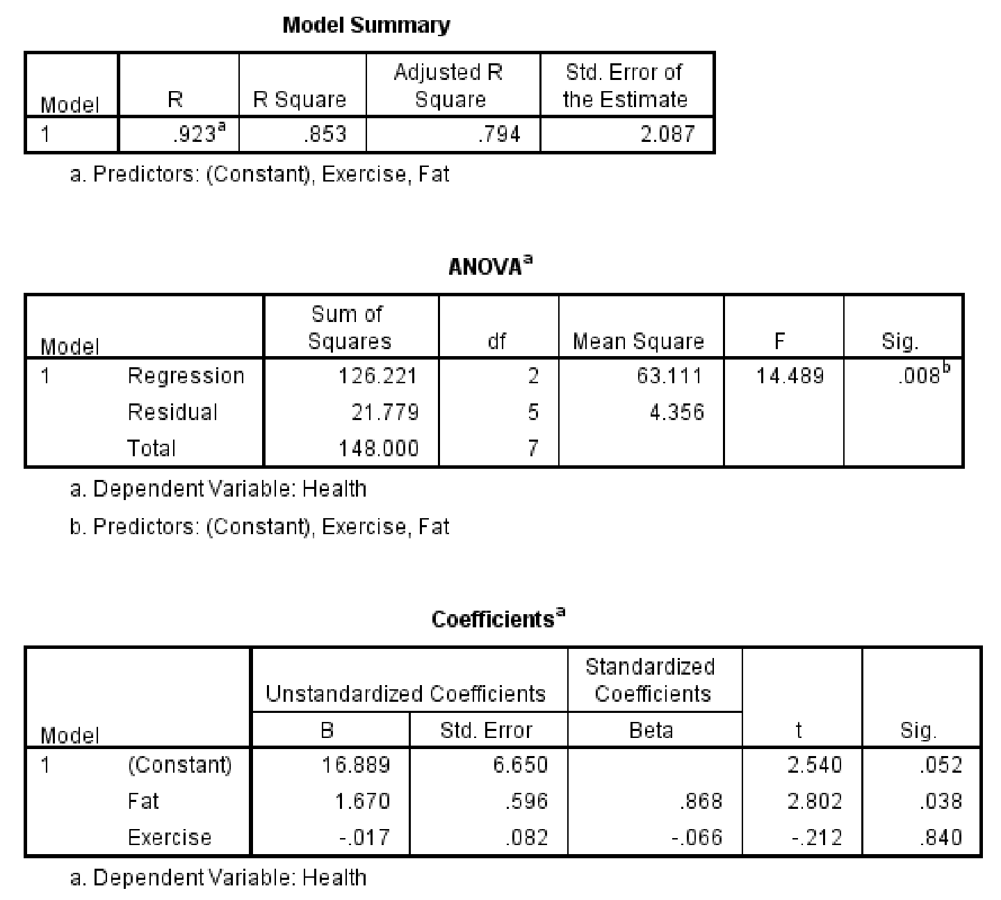
The table of F is,

Source of variation	SS	df	MS	$F_{\text{obt}}$
Regression	126.22	2	63.11	14.48
Residual (error)	21.78	5	4.36
Total	148.00	7

Table 1

Critical value:

The considered significance level is $\alpha =0.05$.

The degrees of freedom for regression are 2, the degrees of freedom for residual are 5.

From the Appendix B: Table B.3-Critical values for F distribution:

• Locate the value 2 in degrees of freedomnumerator row.
• Locate the value 5 in degrees of freedomdenominator row.
• Locate the 0.05 level of significance (value in lightface type) in combined row.
• The intersecting value that corresponds to the (2, 5) with level of significance 0.05 is 5.79.

Thus, the critical value for $df=\left(2,5\right)$ with 0.05, level of significance is 5.79.

Conclusion:

The value of test statistic is 14.48.

The critical value is 5.79.

The test statistic value is greater than the critical value.

The test statistic value falls under critical region.

Hence the null hypothesis is rejected.

Thus, the regression equation significantly predicts variance in criterion variable (Y) health [BMI].

(b)

To determine

Determine which predictor variable or variables, when added to the multiple regression equation, significantly contributed to predictions in Y (health).

Answer to Problem 28CAP

The predictor variable daily intake of fat significantly contributed to predictions in Y (health) when added to the multiple regression equation.

Explanation of Solution

Calculation:

The given information is that, a sample of 8 scores is recorded. The predictor variables are ‘daily intake of fat (in grams) $\left(X_1\right)$’ and ‘amount of exercise (in minutes) $\left(X_2\right)$’ and criterion variable is health (measured using a body mass index [BMI] scale (Y).

Relative contribution to fat$\left(X_1\right)$:

Null hypothesis:

$H_0:$ Adding fat $\left(X_1\right)$ does not improve prediction of variance in Y (health) beyond that already predicted by exercise $\left(X_2\right)$.

Alternative hypothesis:

$H_1:$ Adding fat $\left(X_1\right)$ does improve prediction of variance in Y (health) beyond that already predicted by exercise $\left(X_2\right)$.

The predictor variable fat is tested. The other predictor variable that is not tested is ‘Exercise’. Calculate the correlation between ‘Exercise’ and ‘Health[BMI]’.

Software procedure:

Step by step procedure to obtain correlation using SPSS software is given as,

• Choose Variable view.
• Under the name, enter the name as Health, Exercise.
• Choose Data view, enter the data.
• Choose Analyze>Correlate>Bivariate.
• In variables, enter the Health, and Exercise.
• Click OK.

Output using SPSS software is given below:

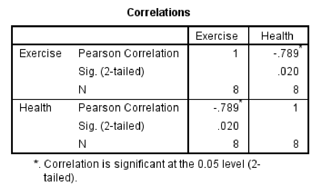
The correlation between ‘Exercise’ and ‘Health [BMI]’ is –0.789.

The value of $r^2$ is,

$\begin{array}{c}{r}^2={\left(-0.789\right)}^2\\ =0.6225\end{array}$

The formula for $S{S}_Y$ is,

$S{S}_Y={\displaystyle \sum Y^2}-\frac{{\left({\displaystyle \sum Y}\right)}^2}{n}$

The calculation of sums of squares is,

Health [BMI] (Y)	$Y^2$
32	1,024
34	1,156
23	529
33	1,089
28	784
27	729
25	625
22	484
${\displaystyle \sum Y}=224$	${\displaystyle \sum Y^2}=6,420$

Table 2

Substitute, ${\displaystyle \sum Y}=224,{\displaystyle \sum Y^2}=6,420,n=8$ in $S{S}_Y$ formula.

$\begin{array}{c}S{S}_Y=6,420-\frac{{\left(224\right)}^2}{8}\\ =6,420-\frac{50,176}{8}\\ =6,420-6,272\\ =148\end{array}$

The contribution of $S{S}_Y$ predicted by ‘Exercise.’ alone is,

$\begin{array}{c}{r}^{2}S{S}_Y=0.6225\times 148\\ =92.13\end{array}$

From the F table, the value of $S{S}_{\text{Regression}}=126.22$, that is the $S{S}_Y$ predicted by ‘Fat $\left(X_1\right)$ and Exercise $\left(X_2\right)$’ is 126.22.

The contribution of $S{S}_Y$ predicted by ‘Fat $\left(X_1\right)$’ alone is,

$\begin{array}{c}S{S}_{\text{Regression}}- S{S}_Y\text{predicted by }\left(X_2\right)=126.22-92.13\\ =34.09\end{array}$

Reproduce the F table by replacing, $S{S}_{\text{Regression}}=126.22$ with $S{S}_Y$ predicted by ‘Fat $\left(X_1\right)$’ alone 34.09.

Since there would be only one predictor variable, the degrees of freedom for regression would be 1.

The mean sums of squares for regression is,

$\begin{array}{c}M{S}_{\text{Regression}}=\frac{S{S}_{\text{Regression}}}{df}\\ =\frac{34.09}{1}\\ =34.09\end{array}$

The F statistic value is,

$\begin{array}{c}{F}_{\text{obt}}=\frac{M{S}_{\text{Regression}}}{M{S}_{\text{Residual}}}\\ =\frac{34.09}{4.36}\\ =7.82\end{array}$

The change F table with $\left(X_1\right)$ alone is,

Source of variation	SS	df	MS	$F_{\text{obt}}$
Regression	34.09	1	34.09	7.82
Residual (error)	21.78	5	4.36
Total	148.00	7

Critical value:

The considered significance level is $\alpha =0.05$.

The degrees of freedom for regression are 1, the degrees of freedom for residual are 5.

From the Appendix B: Table B.3-Critical values for F distribution:

• Locate the value 1 in degrees of freedom numerator row.
• Locate the value 5 in degrees of freedom denominator row.
• Locate the 0.05 level of significance (value in lightface type) in combined row.
• The intersecting value that corresponds to the (1, 5) with level of significance 0.05 is 6.61.

Thus, the critical value for $df=\left(2,5\right)$ with 0.05, level of significance is 6.61.

Conclusion:

The value of test statistic is 7.82.

The critical value is 6.61.

The test statistic value is greater than the critical value.

The test statistic value falls under critical region.

Hence the null hypothesis is rejected.

Thus, adding fat $\left(X_1\right)$ does improve prediction of variance in Y (health) beyond that already predicted by exercise.

Relative contribution to exercise $\left(X_2\right)$:

Null hypothesis:

$H_0:$ Adding exercise $\left(X_2\right)$ does not improve prediction of variance in Y (health) beyond that already predicted by fat $\left(X_1\right)$.

Alternative hypothesis:

$H_1:$ Adding exercise $\left(X_2\right)$ does improve prediction of variance in Y (health) beyond that already predicted by fat $\left(X_1\right)$.

The predictor variable exercise is tested. The other predictor variable that is not tested is ‘fat’. Calculate the correlation between ‘fat’ and ‘Health [BMI]’.

Software procedure:

Step by step procedure to obtain correlation using SPSS software is given as,

• Choose Variable view.
• Under the name, enter the name as Health, Fat.
• Choose Data view, enter the data.
• Choose Analyze>Correlate>Bivariate.
• In variables, enter the Health, and Fat.
• Click OK.

Output using SPSS software is given below:

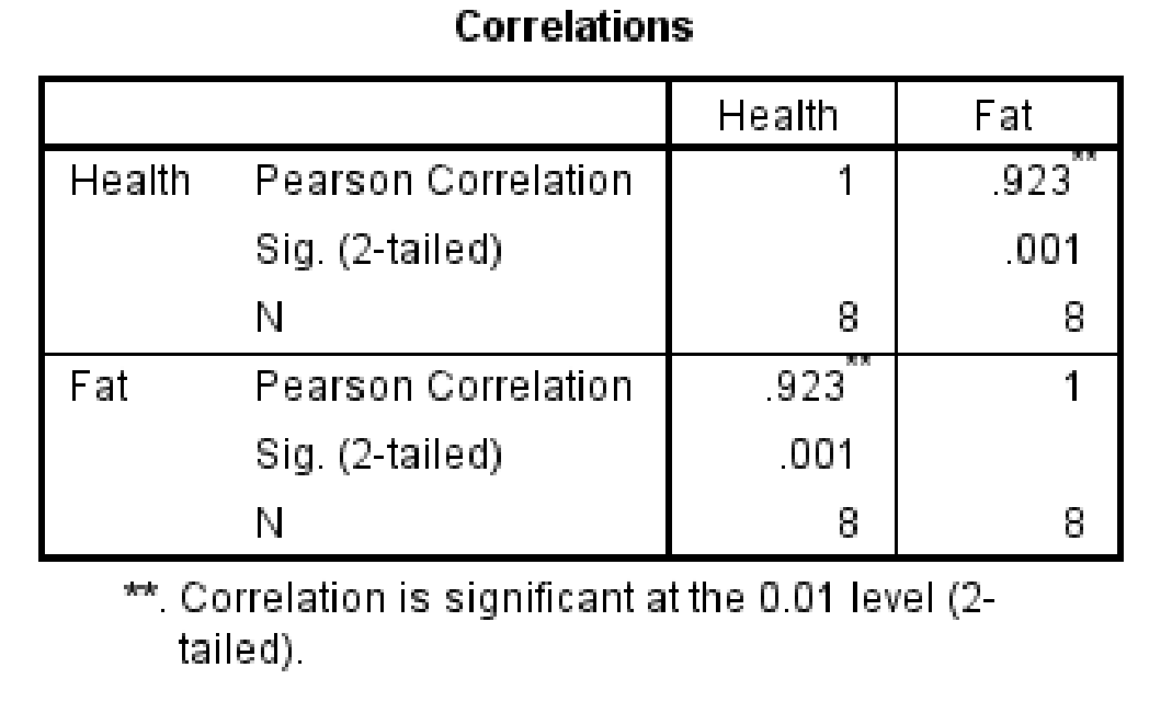
The correlation between ‘fat’ and ‘Health [BMI]’ is 0.923.

The value of $r^2$ is,

$\begin{array}{c}{r}^2={\left(0.923\right)}^2\\ =0.8519\end{array}$

The value for $S{S}_Y$ is calculated as 148. The contribution of $S{S}_Y$ predicted by ‘fat’ alone is,

$\begin{array}{c}{r}^{2}S{S}_Y=0.8519\times 148\\ =126.08\end{array}$

From the F table, the value of $S{S}_{\text{Regression}}=126.22$, that is the $S{S}_Y$ predicted by ‘Fat $\left(X_1\right)$ and Exercise $\left(X_2\right)$’ is 126.22.

The contribution of $S{S}_Y$ predicted by ‘Exercise $\left(X_2\right)$’ alone is,

$\begin{array}{c}S{S}_{\text{Regression}}- S{S}_Y\text{predicted by }\left(X_1\right)=126.22-126.08\\ =0.14\end{array}$

Reproduce the F table by replacing, $S{S}_{\text{Regression}}=126.22$ with $S{S}_Y$ predicted by ‘Exercise $\left(X_2\right)$’ alone 0.14.

Since there would be only one predictor variable, the degrees of freedom for regression would be 1.

The mean sums of squares for regression is,

$\begin{array}{c}M{S}_{\text{Regression}}=\frac{S{S}_{\text{Regression}}}{df}\\ =\frac{0.14}{1}\\ =0.14\end{array}$

The F statistic value is,

$\begin{array}{c}{F}_{\text{obt}}=\frac{M{S}_{\text{Regression}}}{M{S}_{\text{Residual}}}\\ =\frac{0.14}{4.36}\\ =0.03\end{array}$

The change F table with $\left(X_2\right)$ alone is,

Source of variation	SS	df	MS	$F_{\text{obt}}$
Regression	0.14	1	0.14	0.03
Residual (error)	21.78	5	4.36
Total	148.00	7

The critical value for F table with $\left(1,5\right)$ degrees of freedom, at 0.05 significance level is located as 6.61.

Conclusion:

The value of test statistic is 0.03.

The critical value is 6.61.

The test statistic value is less than the critical value.

The test statistic value does not fall under critical region.

Hence the null hypothesis is retained.

Thus, adding exercise $\left(X_2\right)$ does not improve prediction of variance in Y (health) beyond that already predicted by fat $\left(X_1\right)$.

Hence, the predictor variable daily intake of fat significantly contributed to predictions in Y (health) when added to the multiple regression equation.