
Concept explainers
Videos
a.
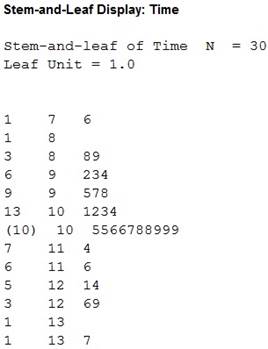
To make: A stem plot for the times customers spent in the restaurant on the next Saturday evening.
a.
Answer to Problem 19.56SE
Explanation of Solution
The given data represent the time spent by the customers in the restaurant on the next Saturday evening. The mean time spent by customers on Saturday evening is 90 minutes and standard deviation is 15 minutes.
Calculation:
Software procedure:
Step-by-step software procedure to draw stemplot using MINITAB software is as follows:
- Select Graph > Stem and leaf.
- Select the column of Time in Graph variables.
- Select OK.
Observation:
Symmetric distribution:
When the left and right sides of the distribution are approximately equal or mirror images of each other, then it is a symmetric distribution.
In the stemplot, the observations of the data set are extended to the left and to the right in a bell shape. Thus, the stemplot shows that data of times are symmetrically distributed.
The
A observation is a suspected outlier, if it is more than
Software procedure:
Step-by-step software procedure for first
- Choose Stat > Basic Statistics > Display
Descriptive Statistics . - In Variables enter the columns Time.
- Choose option statistics, and select first quartile, third quartile, inter quartile
range . - Click OK.
Output using the MINITAB software is as follows:

From Minitab output, the first quartile is 96.50, third quartile is 110.25, and
Substitute IQR in the
The
b.
To check: Whether there is a reason to think that the lavender odor has increased the mean time customers spent in the restaurant or not.
b.
Answer to Problem 19.56SE
Yes, there is a reason to think that the lavender odor has increased the mean time customers spent in the restaurant.
Explanation of Solution
The standard deviation
Calculation:
STATE:
In France, pizza restaurant owner knows the time customers spend in the restaurant on Saturday evening. The mean time spent by the customers in the restaurant is 90 minutes. Is there any reason to think that the lavender odor increased the mean time spent in the restaurant?
PLAN:
Parameter:
Define the parameter
The hypotheses are given below:
The claim of the problem is increase in mean time of customers spent in the restaurant.
Null Hypothesis:
That is, the mean time is equal to 90 minutes.
Alternative hypothesis:
That is, the mean time is greater than 90 minutes. Hence, the alternative hypothesis is one sided.
SOLVE:
Conditions for valid test:
A sample of 20 timings of a restaurant is randomly selected and times follow
Test statistic and P-value:
Software procedure:
Step-by-step procedure to obtain test statistic and P-value using the MINITAB software:
- Choose Stat > Basic Statistics > 1-Sample Z.
- In Samples in Column, enter the column of Times.
- In Standard deviation, enter15.
- In Perform hypothesis test, enter the test mean 90.
- Check Options, enter Confidence level as 95.
- Choose greater than in alternative.
- Click OK in all dialogue boxes.
Output using the MINITAB software is given below:
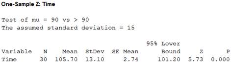
From the MINITAB output, the test statistic is 5.73 and the P-value is 0.000.
Decision criteria for the P-value method:
If
If
CONCLUDE:
Use a significance level,
Here, P-value is 0.000, which is less than the value of
That is,
Therefore, the null hypothesis is rejected.
Thus, there is good evidence that the mean time of customers who spent in the restaurant is increased.
Want to see more full solutions like this?
Chapter 19 Solutions
BASIC PRACTICE OF STATISTICS >C<


 MATLAB: An Introduction with ApplicationsStatisticsISBN:9781119256830Author:Amos GilatPublisher:John Wiley & Sons Inc
 Probability and Statistics for Engineering and th...StatisticsISBN:9781305251809Author:Jay L. DevorePublisher:Cengage Learning
 Statistics for The Behavioral Sciences (MindTap C...StatisticsISBN:9781305504912Author:Frederick J Gravetter, Larry B. WallnauPublisher:Cengage Learning
 Elementary Statistics: Picturing the World (7th E...StatisticsISBN:9780134683416Author:Ron Larson, Betsy FarberPublisher:PEARSON
 The Basic Practice of StatisticsStatisticsISBN:9781319042578Author:David S. Moore, William I. Notz, Michael A. FlignerPublisher:W. H. Freeman
 Introduction to the Practice of StatisticsStatisticsISBN:9781319013387Author:David S. Moore, George P. McCabe, Bruce A. CraigPublisher:W. H. Freeman