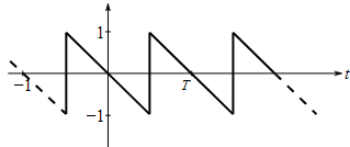
Given Information: The sawtooth wave given in the following figure,
Formula used:
Consider f(t) is a periodic function with period T defined in the interval 0≤x≤T
then the Fourier series expansion of the function,
f(t)=a0+∑k=1∞[akcos(kω0t)+bksin(kω0t)] with ω0=2πT.
And the coefficients are defined by,
a0=1T∫0Tf(t)dt ; ak=2T∫0Tf(t)cos(kω0t)dt ; bk=2T∫0Tf(t)sin(kω0t)dt
Alternatively, the Fourier series can also be written as, f(t)=a0+∑k=1∞[ckcos(kω0t−ϕk)]
Here, the amplitude ck and phase ϕk for each term is defined as,
ck2=ak2+bk2,ϕk=tan−1(bkak)
Plot ck and ϕk in the frequency domain to plot the amplitude and phase line spectra.
Graph:
Consider the sawtooth wave given in the following figure,
Therefore, the sawtooth wave is a periodic function f(t) with period T in the interval 0≤t≤T and from the graph,
f(t) is a straight line joining the points (0,0) and (T2,−1) in 0≤t≤T2.
f(t) is a straight line joining the points (T2,1) and (T,0) in T2≤t≤T.
Therefore, the sawtooth wave,
f(t)={−2Tt0≤t≤T22−2TtT2≤t≤T
Therefore, the Fourier series expansion of this function is,
f(t)=a0+∑k=1∞[akcos(kω0t)+bksin(kω0t)];ω0=2πT
In the above expression, the coefficients are defined by,
Now, find ak.
ak=2T∫0Tf(t)cos(2kπTt)dt=2T∫0T2(−2Tt)cos(2kπTt)dt+2T∫T2T(2−2Tt)cos(2kπTt)dt=−4T2∫0T2tcos(2kπTt)dt+4T∫T2Tcos(2kπTt)dt−4T2∫T2Ttcos(2kπTt)dt
Consider,
I=∫tcos(2kπTt)dt=t∫cos(2kπTt)dt−∫{ddt(t)∫cos(2kπTt)dt}dt=tT2kπsin(2kπTt)−∫T2kπsin(2kπTt)dt=Tt2kπsin(2kπTt)+T24k2π2cos(2kπTt)
Hence,
∫0T2tcos(2kπTt)dt=[Tt2kπsin(2kπTt)+T24k2π2cos(2kπTt)]0T2=T2kπT2sin(2kπTT2)+T24k2π2cos(2kπTT2)−T24k2π2cos(0)=T24kπsin(kπ)+T24k2π2cos(kπ)−T24k2π2=T24k2π2(−1)k−T24k2π2
Further,
∫T2Tcos(2kπTt)dt=T2kπsin(2kπTt)|T2T=T2kπ{sin(2kπ)−sin(kπ)}=0
∫T2Ttcos(2kπTt)dt=[Tt2kπsin(2kπTt)+T24k2π2cos(2kπTt)]T2T=T22kπsin(2kπ)+T24k2π2cos(2kπ)−T24kπsin(kπ)−T24k2π2cos(kπ)=T24k2π2−T24k2π2(−1)k
Therefore,
ak=−4T2[T24k2π2(−1)k−T24k2π2]+4T×0−4T2[T24k2π2−T24k2π2(−1)k]=−1k2π2(−1)k+1k2π2−1k2π2+1k2π2(−1)k=0
Now, find bk.
bk=2T∫0Tf(t)sin(2kπTt)dt=2T∫0T2(−2Tt)sin(2kπTt)dt+2T∫T2T(2−2Tt)sin(2kπTt)dt=−4T2∫0T2tsin(2kπTt)dt+4T∫T2Tsin(2kπTt)dt−4T2∫T2Ttsin(2kπTt)dt
Consider,
I=∫tsin(2kπTt)dt=t∫sin(2kπTt)dt−∫{ddt(t)∫sin(2kπTt)dt}dt=−tT2kπcos(2kπTt)+∫T2kπcos(2kπTt)dt=−Tt2kπcos(2kπTt)+T24k2π2sin(2kπTt)
Hence,
∫0T2tsin(2kπTt)dt=[−Tt2kπcos(2kπTt)+T24k2π2sin(2kπTt)]0T2=−T24kπcos(kπ)+T24k2π2sin(kπ)=−T24kπ(−1)k
∫T2Tsin(2kπTt)dt=−T2kπcos(2kπTt)|T2T=−T2kπcos(2kπ)+T2kπcos(kπ)=−T2kπ+T2kπ(−1)k
Further,
∫T2Ttsin(2kπTt)dt=[−Tt2kπcos(2kπTt)+T24k2π2sin(2kπTt)]T2T=−T22kπcos(2kπ)+T24k2π2sin(2kπ)+T24kπcos(kπ)−T24k2π2sin(kπ)=−T22kπ+T24kπ(−1)k
Thus,
bk=−4T2[−T24kπ(−1)k]+4T[−T2kπ+T2kπ(−1)k]−4T2[−T22kπ+T24kπ(−1)k]=1kπ(−1)k−2kπ+2kπ(−1)k+2kπ−1kπ(−1)k=2kπ(−1)k
Hence, the coefficients of the Fourier series expansions are,
a0=0,ak=0,bk=2kπ(−1)k
That is,
bk={2kπ>0k even−2kπ<0k odd
Consider,
ck=ak2+bk2=0+4k2π2(−1)2k=4k2π2=2kπ
Thus, the amplitude of the kth term is 2kπ, that is, the amplitudes for k=1,2,3,4,5,... are,
2π,1π,23π,12π,25π,...
Furthermore, consider,
ϕk=tan−1(bkak)
As ak=0 and bk>0 for even k thus,
ϕk=π2
As ak=0 and bk<0 for odd k thus,
ϕk=−π2
Therefore,
ϕk={π2k even−π2k odd
Thus, the phases corresponding to k=1,2,3,4,5,... are −π2,π2,−π2,π2,−π2,...
Use the following MATLAB code to construct the amplitude plot.
function Code_97924_19_6P_a()
for k = 1: 8
f(k) = k;
% define the amplitude
A(k) = 2/(k*pi);
end
% plot the values thus obtained
stem(f,A,'filled','LineWidth',4,'Color','k','Marker', 'none');
% define geometric properties
set(gca,'XTickLabel',{' ' 'f_0' 'f_1' 'f_2' 'f_3' 'f_4' 'f_5' 'f_6' 'f_7'});
set(gca,'YTick',[A(8) A(4) A(2) A(1)]);
set(gca,'YTickLabel',{'1/4\pi' '1/2\pi' '1/\pi' '2/\pi'});
set(gca,'Fontname','Times New Roman','FontSize',12);
xlim([0, 9]); grid on
end
Execute the above code to obtain the amplitude plot as,
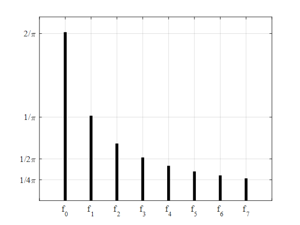
Interpretation: The above plot shows the amplitude plot for the sawtooth wave as shown in the figure provided.
Use the following MATLAB file can be used to construct the phase plot.
function Code_97924_19_6P_b()
for k = 1: 8
f(k) = k;
% define the phase
P(k) = (-1)^k*(pi/2);
end
% plot the values thus obtained
stem(f,P,'filled','LineWidth',4,'Color','k','Marker', 'none');
% define geometric properties
set(gca,'XTickLabel',{' ' 'f_0' 'f_1' 'f_2' 'f_3' 'f_4' 'f_5' 'f_6' 'f_7'});
set(gca,'YTick',[-pi -pi/2 0 pi/2 pi]);
set(gca,'YTickLabel',{'-\pi' '-\pi/2' '0' '\pi/2' '\pi'});
set(gca,'Fontname','Times New Roman','FontSize',12);
xlim([0, 9]); grid on
ylim([-pi-0.1, pi+0.1]); grid on
end
Execute the above code to obtain the plot as,
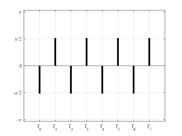
Interpretation: The above plot shows the phase line spectra for the sawtooth wave as shown in the figure provided.


 Trigonometry (MindTap Course List)TrigonometryISBN:9781337278461Author:Ron LarsonPublisher:Cengage Learning
 Algebra & Trigonometry with Analytic GeometryAlgebraISBN:9781133382119Author:SwokowskiPublisher:Cengage
 Trigonometry (MindTap Course List)TrigonometryISBN:9781305652224Author:Charles P. McKeague, Mark D. TurnerPublisher:Cengage Learning