ETSU PRACSTAT + SAP ACESS 12MO (LL)
8th Edition
ISBN: 9781319226145
Author: Moore
Publisher: Macmillan Higher Education
bartleby

Concept explainers

bartleby

Videos

Question
Book Icon
Chapter 2, Problem 144E

(a)

To determine

To graph: The scatterplot.

(a)

Expert Solution
Check Mark

Explanation of Solution

Graph: To draw the scatterplot for the provided data set, the below steps are followed in Minitab software.

Step 1: Open the “MEIS” file in Minitab software.

Step 2: Go to Graph Scatterplot.

Step 3: Choose the option “Simple” and click “OK”.

Step 4: Select “Sales” as Y variables and “Dwellpermit” as X variables.

Step 5: Click “OK” twice.

The scatterplot is obtained as:

ETSU PRACSTAT + SAP ACESS 12MO (LL), Chapter 2, Problem 144E , additional homework tip  1

To determine

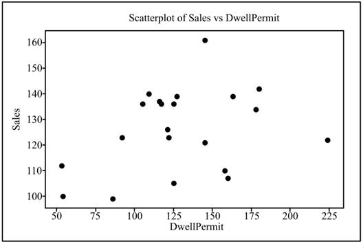
To explain: The relationship between the variables and the presence of the outliers.

Expert Solution
Check Mark

Answer to Problem 144E

Solution: Though the relationship between the variables is very weak, but there is no outlier in the data set.

Explanation of Solution

The scatterplot obtained in part (a) shows that the data are very much scattered. That is there is very weak relationship between the response variable sales and the explanatory variable, issued permits. But there is no outlier present in the data set.

(b)

To determine

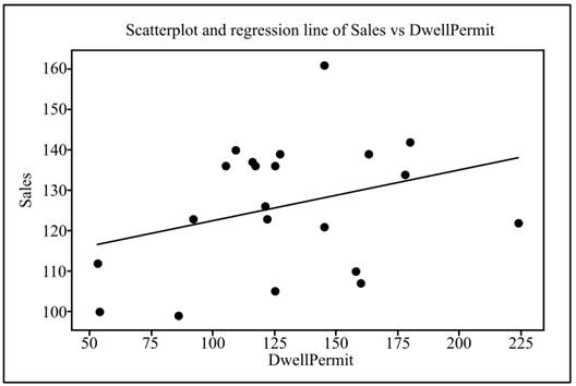
To find: The least-squares regression line for the data.

(b)

Expert Solution
Check Mark

Answer to Problem 144E

Solution: The least-squares regression line is obtained as Sales=109.8+0.1263DwellPermit, which is shown in the below diagram.

ETSU PRACSTAT + SAP ACESS 12MO (LL), Chapter 2, Problem 144E , additional homework tip  2

Explanation of Solution

Calculation: To draw the regression line and obtain the sketch of the regression line, the below steps are followed in the Minitab software.

Step 1: Right click on the obtained graph in the part (a).

Step 2: Go to Add Regression Fit.

Step 3: Click on “Linear” under the menu “Model Order” and tick the “Fit intercept”.

Step 4: Click on “OK” to obtain the regression line.

The obtained regression equation is Sales=109.8+0.1263DwellPermit.

Graph: The below graph shows the regression line.

ETSU PRACSTAT + SAP ACESS 12MO (LL), Chapter 2, Problem 144E , additional homework tip  3

(c)

To determine

To explain: The slope of the obtained line.

(c)

Expert Solution
Check Mark

Answer to Problem 144E

Solution: The slope can be interpreted as if there is an increase of 1unit of the variable, issued permit for dwelling then there is an increase of 0.1263 units in the value of the variable sales.

Explanation of Solution

The slope of the least-square regression line indicates the amount of increase (decrease) in the response variable due to the 1-unit increase (decrease) in the value of the explanatory variable. In the provided equation, the amount of increase in the value of the response variable, sales is 0.1263 due to the 1-unit increase in the value of the variable issued permit for dwelling.

(d)

To determine

To explain: The intercept of the line.

(d)

Expert Solution
Check Mark

Answer to Problem 144E

Solution: The intercept can be interpreted as the value of the response variable when the value of the explanatory variable is zero. As the value of the response variable is 109.8 for the zero issued permits, it is appropriate to use the intercept for explaining the relationship between the variables.

Explanation of Solution

The intercept of the least-squares linear regression provided the value of the response variable when the value of the explanatory variable is zero. The explanatory variable can be zero because the index of issued permits for new dwelling can be zero and the value of the response variable for zero issued permit is 109.8. Therefore, it is appropriate to use the intercept for explaining the relationship between the variables.

(e)

To determine

The sales for an index of 224 dwelling permits.

(e)

Expert Solution
Check Mark

Answer to Problem 144E

Solution: The predicted value of the sales is 138.0912.

Explanation of Solution

The predicted value of the sales can be obtained by substituting the value of the index of dwelling permit in the least-squares linear regression equation.

The predicted value can be calculated as:

Sales=109.8+0.1263DwellPermit=109.8+0.1263×224=138.0912

(f)

To determine

To find: The residual value for Canada.

(f)

Expert Solution
Check Mark

Answer to Problem 144E

Solution: The obtained value of the residual is 8.0912_.

Explanation of Solution

Calculation: The sale for the Canada is provided as 122. The residual value for the sales for Canada whose index of dwelling permits is 224 is calculated as:

Residual=Observed SalesPredicted Sales=122138.0912=16.0912

(g)

To determine

The percentage of variability in sales is explained by dwelling permit.

(g)

Expert Solution
Check Mark

Answer to Problem 144E

Solution: The explained percentage of variability in sales is 10.30%.

Explanation of Solution

The variability is explained by r2 which indicates that how better the model fits the data. The value of r2 is obtained along with the regression line when the line is added to the obtained scatterplot in the Minitab software in part (b). The value is obtained as 10.30%.

Therefore, the proportion of variation that is explained by the explanatory variables of the model is 10.30%.

Want to see more full solutions like this?

Subscribe now to access step-by-step solutions to millions of textbook problems written by subject matter experts!

Chapter 2 Solutions

ETSU PRACSTAT + SAP ACESS 12MO (LL)

Ch. 2.2 - Prob. 11UYKCh. 2.2 - Prob. 12UYKCh. 2.2 - Prob. 13UYKCh. 2.2 - Prob. 14UYKCh. 2.2 - Prob. 15UYKCh. 2.2 - Prob. 16ECh. 2.2 - Prob. 17ECh. 2.2 - Prob. 18ECh. 2.2 - Prob. 19ECh. 2.2 - Prob. 20ECh. 2.2 - Prob. 21ECh. 2.2 - Prob. 22ECh. 2.2 - Prob. 23ECh. 2.2 - Prob. 24ECh. 2.2 - Prob. 25ECh. 2.2 - Prob. 26ECh. 2.2 - Prob. 27ECh. 2.2 - Prob. 28ECh. 2.2 - Prob. 29ECh. 2.2 - Prob. 30ECh. 2.2 - Prob. 31ECh. 2.2 - Prob. 32ECh. 2.2 - Prob. 33ECh. 2.2 - Prob. 34ECh. 2.2 - Prob. 35ECh. 2.2 - Prob. 36ECh. 2.2 - Prob. 37ECh. 2.3 - Prob. 38UYKCh. 2.3 - Prob. 39UYKCh. 2.3 - Prob. 40ECh. 2.3 - Prob. 41ECh. 2.3 - Prob. 42ECh. 2.3 - Prob. 43ECh. 2.3 - Prob. 44ECh. 2.3 - Prob. 45ECh. 2.3 - Prob. 46ECh. 2.3 - Prob. 47ECh. 2.3 - Prob. 48ECh. 2.3 - Prob. 49ECh. 2.3 - Prob. 50ECh. 2.3 - Prob. 51ECh. 2.3 - Prob. 52ECh. 2.3 - Prob. 53ECh. 2.3 - Prob. 54ECh. 2.3 - Prob. 55ECh. 2.3 - Prob. 56ECh. 2.3 - Prob. 57ECh. 2.3 - Prob. 58ECh. 2.3 - Prob. 59ECh. 2.3 - Prob. 60ECh. 2.4 - Prob. 61UYKCh. 2.4 - Prob. 62UYKCh. 2.4 - Prob. 63UYKCh. 2.4 - Prob. 64UYKCh. 2.4 - Prob. 65ECh. 2.4 - Prob. 66ECh. 2.4 - Prob. 67ECh. 2.4 - Prob. 68ECh. 2.4 - Prob. 69ECh. 2.4 - Prob. 70ECh. 2.4 - Prob. 71ECh. 2.4 - Prob. 72ECh. 2.4 - Prob. 73ECh. 2.4 - Prob. 74ECh. 2.4 - Prob. 75ECh. 2.4 - Prob. 76ECh. 2.4 - Prob. 77ECh. 2.4 - Prob. 78ECh. 2.4 - Prob. 79ECh. 2.4 - Prob. 80ECh. 2.4 - Prob. 81ECh. 2.4 - Prob. 82ECh. 2.4 - Prob. 83ECh. 2.4 - Prob. 84ECh. 2.4 - Prob. 85ECh. 2.4 - Prob. 86ECh. 2.4 - Prob. 87ECh. 2.4 - Prob. 88ECh. 2.4 - Prob. 89ECh. 2.4 - Prob. 90ECh. 2.4 - Prob. 91ECh. 2.5 - Prob. 92UYKCh. 2.5 - Prob. 93UYKCh. 2.5 - Prob. 94ECh. 2.5 - Prob. 95ECh. 2.5 - Prob. 96ECh. 2.5 - Prob. 97ECh. 2.5 - Prob. 98ECh. 2.5 - Prob. 99ECh. 2.5 - Prob. 100ECh. 2.5 - Prob. 101ECh. 2.5 - Prob. 102ECh. 2.5 - Prob. 103ECh. 2.5 - Prob. 104ECh. 2.5 - Prob. 105ECh. 2.5 - Prob. 106ECh. 2.5 - Prob. 107ECh. 2.5 - Prob. 108ECh. 2.5 - Prob. 110ECh. 2.5 - Prob. 111ECh. 2.5 - Prob. 112ECh. 2.6 - Prob. 113UYKCh. 2.6 - Prob. 114UYKCh. 2.6 - Prob. 115UYKCh. 2.6 - Prob. 116UYKCh. 2.6 - Prob. 117UYKCh. 2.6 - Prob. 118UYKCh. 2.6 - Prob. 119ECh. 2.6 - Prob. 120ECh. 2.6 - Prob. 121ECh. 2.6 - Prob. 122ECh. 2.6 - Prob. 123ECh. 2.6 - Prob. 124ECh. 2.6 - Prob. 125ECh. 2.6 - Prob. 126ECh. 2.6 - Prob. 127ECh. 2.6 - Prob. 128ECh. 2.6 - Prob. 129ECh. 2.6 - Prob. 130ECh. 2.7 - Prob. 131ECh. 2.7 - Prob. 132ECh. 2.7 - Prob. 133ECh. 2.7 - Prob. 134ECh. 2.7 - Prob. 135ECh. 2.7 - Prob. 136ECh. 2.7 - Prob. 137ECh. 2.7 - Prob. 138ECh. 2.7 - Prob. 139ECh. 2.7 - Prob. 140ECh. 2.7 - Prob. 141ECh. 2.7 - Prob. 142ECh. 2.7 - Prob. 143ECh. 2 - Prob. 144ECh. 2 - Prob. 145ECh. 2 - Prob. 146ECh. 2 - Prob. 147ECh. 2 - Prob. 148ECh. 2 - Prob. 149ECh. 2 - Prob. 150ECh. 2 - Prob. 151ECh. 2 - Prob. 152ECh. 2 - Prob. 153ECh. 2 - Prob. 154ECh. 2 - Prob. 155ECh. 2 - Prob. 156ECh. 2 - Prob. 157ECh. 2 - Prob. 158ECh. 2 - Prob. 159ECh. 2 - Prob. 160ECh. 2 - Prob. 161ECh. 2 - Prob. 162ECh. 2 - Prob. 163ECh. 2 - Prob. 164ECh. 2 - Prob. 165ECh. 2 - Prob. 166ECh. 2 - Prob. 167ECh. 2 - Prob. 168ECh. 2 - Prob. 169ECh. 2 - Prob. 170ECh. 2 - Prob. 171ECh. 2 - Prob. 172ECh. 2 - Prob. 173ECh. 2 - Prob. 174ECh. 2 - Prob. 175ECh. 2 - Prob. 176E
Knowledge Booster
Background pattern image
Statistics
Learn more about
Need a deep-dive on the concept behind this application? Look no further. Learn more about this topic, statistics and related others by exploring similar questions and additional content below.
Recommended textbooks for you
Text book image
MATLAB: An Introduction with Applications
Statistics
ISBN:9781119256830
Author:Amos Gilat
Publisher:John Wiley & Sons Inc
Text book image
Probability and Statistics for Engineering and th...
Statistics
ISBN:9781305251809
Author:Jay L. Devore
Publisher:Cengage Learning
Text book image
Statistics for The Behavioral Sciences (MindTap C...
Statistics
ISBN:9781305504912
Author:Frederick J Gravetter, Larry B. Wallnau
Publisher:Cengage Learning
Text book image
Elementary Statistics: Picturing the World (7th E...
Statistics
ISBN:9780134683416
Author:Ron Larson, Betsy Farber
Publisher:PEARSON
Text book image
The Basic Practice of Statistics
Statistics
ISBN:9781319042578
Author:David S. Moore, William I. Notz, Michael A. Fligner
Publisher:W. H. Freeman
Text book image
Introduction to the Practice of Statistics
Statistics
ISBN:9781319013387
Author:David S. Moore, George P. McCabe, Bruce A. Craig
Publisher:W. H. Freeman
The Shape of Data: Distributions: Crash Course Statistics #7; Author: CrashCourse;https://www.youtube.com/watch?v=bPFNxD3Yg6U;License: Standard YouTube License, CC-BY
Shape, Center, and Spread - Module 20.2 (Part 1); Author: Mrmathblog;https://www.youtube.com/watch?v=COaid7O_Gag;License: Standard YouTube License, CC-BY
Shape, Center and Spread; Author: Emily Murdock;https://www.youtube.com/watch?v=_YyW0DSCzpM;License: Standard Youtube License