Chapter 2, Problem 178E

To determine

To find: A scatterplot of the provided data of 50 states with variables related to health conditions and risk behavior as well as demographic information and to find the numerical summaries of the provided data and to write a short report on the data.

Answer to Problem 178E

Solution: For the pair of variables: (EdCollege, Female), the coefficient of determination value is $R^2=0.021$.

For the pair of variables: (EdCollege, Age 18-24), the coefficient of determination value is $R^2=0.014$.

For the pair of variables: (EdCollege, Age 25-34), the coefficient of determination value is $R^2=0.03$.

Explanation of Solution

Given: The data of 50 states with variables related to health conditions and risk behavior as well as demographic information is provided in the question.

State	Age18_24	Age25_34	Female	EdCollege
Alabama	13.0	17.1	52.3	19.7
Alaska	14.6	20.7	48.2	23.7
Arizona	12.5	19.2	50.4	23.7
Arkansas	12.6	17.7	51.7	17.4
California	13.4	19.3	50.4	27.0
Colorado	12.7	18.2	49.9	32.6
Connecticut	12.3	15.2	51.9	32.5
Delaware	12.1	16.8	52.3	25.3
District of Columbia	13.9	23.0	53.7	45.2
Florida	11.3	16.2	51.4	23.8
Georgia	13.4	18.8	51.4	24.6
Guam	16.9	19.6	49.0	26.0
Hawaii	11.9	18.8	50.0	26.7
Idaho	14.1	18.4	50.2	21.7
Illinois	13.2	18.0	51.3	27.8
Indiana	13.4	17.1	51.3	20.5
Iowa	13.6	16.0	51.1	22.6
Kansas	14.0	17.5	50.9	26.5
Kentucky	12.5	17.3	51.6	18.7
Louisiana	13.8	18.6	52.2	18.9
Maine	11.1	14.3	51.8	24.5
Maryland	12.3	17.3	52.3	32.8
Massachusetts	12.7	16.6	52.1	35.4
Michigan	13.1	15.7	51.4	22.8
Minnesota	12.8	17.4	50.7	28.8
Mississippi	14.4	17.9	52.3	17.5
Missouri	12.9	17.2	51.8	23.0
Montana	12.9	15.8	50.3	25.1
Nebraska	14.2	17.4	50.9	25.2
Nevada	11.7	19.5	49.4	19.9
New Hampshire	12.4	14.5	51.2	30.2
New Jersey	11.3	16.4	51.6	32.3
New Mexico	13.1	18.6	51.0	22.7
New York	12.5	17.4	52.1	29.9
North Carolina	12.9	17.2	51.7	23.8
North Dakota	16.8	16.8	50.0	23.6
Ohio	12.3	16.6	51.9	22.3
Oklahoma	13.8	18.2	51.2	20.4
Oregon	12.2	16.3	50.8	26.1
Pennsylvania	12.3	15.6	52.0	24.5
Puerto Rico	14.6	19.2	53.1	19.4
Rhode Island	13.2	15.9	52.2	27.5
South Carolina	12.8	17.1	52.1	21.8
South Dakota	13.9	17.0	50.4	22.9
Tennessee	12.1	17.3	51.9	20.9
Texas	13.9	19.7	50.6	23.1
Utah	17.2	22.8	50.1	25.4
Vermont	13.2	14.2	51.3	30.2
Virginia	12.9	17.2	51.3	30.9

Calculation: From the given data set consider the following three pair of variables.

1. EdCollege and Female

2. EdCollege and Age 18-24

3. EdCollege and Age 25-34

Now, construct the scatterplot with fitted linear regression line for each pair of variables.

Use Minitab to get the required result.

To draw the scatterplot of the provided data, below mentioned steps are followed in Minitab.

Step 1: Enter the data into Minitab worksheet.

Step 2: Go to Graph, select scatterplot and linear regression and click OK.

Step 3: Select the data variable column and click on Scale.

Step 4: Check minor ticks under Y Scale Low and X Scale Low and then click OK.

The obtained scatterplot of EdCollege and Female is shown below:

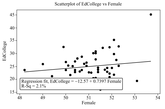
From the above plot we observe that there is a low positive relation between the two variables female and EdCollege.

The regression fit for the data is $y=-12.57+0.7397x$.

The obtained scatterplot of EdCollege and Age 18-24 is shown below.

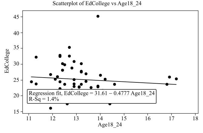
From the above plot we observe that there is a low negative relation between the two variables Age 18-24 and EdCollege. The regression fit for the data is $y=31.61-0.4777x$.

The obtained scatterplot of EdCollege and Age 25-34 is shown below.

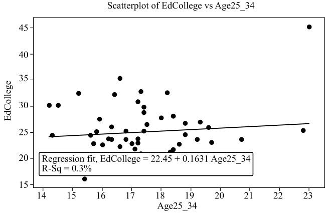
From the above plot we observe that there is a low positive relation between the two variables Age 25-34 and EdCollege.

The regression fit for the data is $y=22.45+0.1631x$.

Interpretation: Consider the first pair of variables, EdCollege and Female. The coefficient of determination value is $R^2=0.021$, this means that only 2.1% of the variation is explained by the independent variable and remaining by the dependent variable.

Consider second pair of variables, EdCollege and Age 18-24. The coefficient of determination value is $R^2=0.014$, this means that only 1.4% of the variation is explained by the independent variable and remaining by the dependent variable.

Consider third pair of variables, EdCollege and Age 25-34. The coefficient of determination value is $R^2=0.03$, this means that only 0.3% of the variation is explained by the independent variable and remaining by the dependent variable.