Chapter 2, Problem 54SE

a.

To determine

Construct a cross tabulation with Year founded and % Graduate.

Answer to Problem 54SE

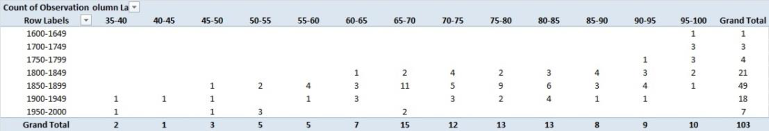
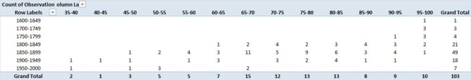
The cross tabulation with Year founded and % Graduate is given below.

Explanation of Solution

Calculation:

The given data represents sample of 103 private colleges and universities.

The cross tabulation for the data on Year founded as row variable and % Graduate as the column variable is computed below.

Software procedure:

Step-by-step procedure to develop a cross tabulation using EXCEL:

• Select Insert > Tables > PivotTable.
• In Create PivotTable, select Table/Range and click Ok.
• In PivotTable Fields, drag Year founded to ROWS, % Graduate to COLUMNS, and observations to VALUES.
• Click on Sum of Observations > Value field settings.
• In Value Field Settings, select Count under Summarize value field by.
• Click OK.
• Right click on any of the row variables and select Group.
• In Grouping, give 1,600 in Starting at, 2,000 in Ending at, and 50 in By.
• Click Ok.
• Right click on any of the column variables and select Group.
• In Grouping, give 35 in Starting at, 100 in Ending at, and 5 in By.
• Click Ok.

The EXCEL output is given below:

b.

To determine

Compute row percentages for the cross tabulation obtained in Part (a).

Answer to Problem 54SE

The row percentages for the cross tabulation in Part (a) is given below.

Year founded	35–40	40–45	45–50	50–55	55–60	60–65	65–70
1600–1649	0	0	0	0	0	0	0
1700–1749	0	0	0	0	0	0	0
1750–1799	0	0	0	0	0	0	0
1800–1849	0	0	0	0	0	4.76	9.52
1850–1899	0	0	2.04	4.08	8.16	6.12	22.45
1900–1949	5.56	5.56	5.56	0	5.56	16.67	0
1950–2000	14.29	0	14.29	42.86	0	0	28.57

Year founded	70–75	75–80	80–85	85–90	90–95	95–100	Total
1600–1649	0	0	0	0	0	100	100
1700–1749	0	0	0	0	0	100	100
1750–1799	0	0	0	0	25	75	100
1800–1849	19.05	9.52	14.29	19.05	14.29	9.52	100
1850–1899	10.2	18.37	12.24	6.12	8.16	2.04	100
1900–1949	16.67	11.11	22.22	5.56	5.56	0	100
1950–2000	0	0	0	0	0	0	100

Explanation of Solution

Calculation:

Dividing each frequency by its row margin and multiplying it with 100 gives row percentages.

The row percentage for the cross tabulation in Part (a) is calculated below.

Year founded	35–40	40–45	45–50	50–55	55–60	60–65	65–70
1600–1649	$\begin{array}{r}\frac{0}{1}\times 100\\ =0\end{array}$	$\begin{array}{r}\frac{0}{1}\times 100\\ =0\end{array}$	$\begin{array}{r}\frac{0}{1}\times 100\\ =0\end{array}$	$\begin{array}{r}\frac{0}{1}\times 100\\ =0\end{array}$	$\begin{array}{r}\frac{0}{1}\times 100\\ =0\end{array}$	$\begin{array}{r}\frac{0}{1}\times 100\\ =0\end{array}$	$\begin{array}{r}\frac{0}{1}\times 100\\ =0\end{array}$
1700–1749	$\begin{array}{r}\frac{0}{3}\times 100\\ =0\end{array}$	$\begin{array}{r}\frac{0}{3}\times 100\\ =0\end{array}$	$\begin{array}{r}\frac{0}{3}\times 100\\ =0\end{array}$	$\begin{array}{r}\frac{0}{3}\times 100\\ =0\end{array}$	$\begin{array}{r}\frac{0}{3}\times 100\\ =0\end{array}$	$\begin{array}{r}\frac{0}{3}\times 100\\ =0\end{array}$	$\begin{array}{r}\frac{0}{3}\times 100\\ =0\end{array}$
1750–1799	$\begin{array}{r}\frac{0}{4}\times 100\\ =0\end{array}$	$\begin{array}{r}\frac{0}{4}\times 100\\ =0\end{array}$	$\begin{array}{r}\frac{0}{4}\times 100\\ =0\end{array}$	$\begin{array}{r}\frac{0}{4}\times 100\\ =0\end{array}$	$\begin{array}{r}\frac{0}{4}\times 100\\ =0\end{array}$	$\begin{array}{r}\frac{0}{4}\times 100\\ =0\end{array}$	$\begin{array}{r}\frac{0}{4}\times 100\\ =0\end{array}$
1800–1849	$\begin{array}{r}\frac{0}{21}\times 100\\ =0\end{array}$	$\begin{array}{r}\frac{0}{21}\times 100\\ =0\end{array}$	$\begin{array}{r}\frac{0}{21}\times 100\\ =0\end{array}$	$\begin{array}{r}\frac{0}{21}\times 100\\ =0\end{array}$	$\begin{array}{r}\frac{0}{21}\times 100\\ =0\end{array}$	$\begin{array}{r}\frac{1}{21}\times 100\\ =4.76\end{array}$	$\begin{array}{r}\frac{2}{21}\times 100\\ =9.52\end{array}$
1850–1899	$\begin{array}{r}\frac{0}{49}\times 100\\ =0\end{array}$	$\begin{array}{r}\frac{0}{49}\times 100\\ =0\end{array}$	$\begin{array}{r}\frac{1}{49}\times 100\\ =2.04\end{array}$	$\begin{array}{r}\frac{2}{49}\times 100\\ =4.08\end{array}$	$\begin{array}{r}\frac{4}{49}\times 100\\ =8.16\end{array}$	$\begin{array}{r}\frac{3}{49}\times 100\\ =6.12\end{array}$	$\begin{array}{r}\frac{11}{49}\times 100\\ =22.45\end{array}$
1900–1949	$\begin{array}{r}\frac{1}{18}\times 100\\ =5.56\end{array}$	$\begin{array}{r}\frac{1}{18}\times 100\\ =5.56\end{array}$	$\begin{array}{r}\frac{1}{18}\times 100\\ =5.56\end{array}$	$\begin{array}{r}\frac{0}{18}\times 100\\ =0\end{array}$	$\begin{array}{r}\frac{1}{18}\times 100\\ =5.56\end{array}$	$\begin{array}{r}\frac{3}{18}\times 100\\ =16.67\end{array}$	$\begin{array}{r}\frac{0}{18}\times 100\\ =0\end{array}$
1950–2000	$\begin{array}{r}\frac{1}{7}\times 100\\ =14.29\end{array}$	$\begin{array}{r}\frac{0}{7}\times 100\\ =0\end{array}$	$\begin{array}{r}\frac{1}{7}\times 100\\ =14.29\end{array}$	$\begin{array}{r}\frac{3}{7}\times 100\\ =42.86\end{array}$	$\begin{array}{r}\frac{0}{7}\times 100\\ =0\end{array}$	$\begin{array}{r}\frac{0}{7}\times 100\\ =0\end{array}$	$\begin{array}{r}\frac{2}{7}\times 100\\ =28.57\end{array}$

Year founded	70–75	75–80	80–85	85–90	90–95	95–100	Total
1600–1649	$\begin{array}{r}\frac{0}{1}\times 100\\ =0\end{array}$	$\begin{array}{r}\frac{0}{1}\times 100\\ =0\end{array}$	$\begin{array}{r}\frac{0}{1}\times 100\\ =0\end{array}$	$\begin{array}{r}\frac{0}{1}\times 100\\ =0\end{array}$	$\begin{array}{r}\frac{0}{1}\times 100\\ =0\end{array}$	$\begin{array}{r}\frac{1}{1}\times 100\\ =100\end{array}$	100
1700–1749	$\begin{array}{r}\frac{0}{3}\times 100\\ =0\end{array}$	$\begin{array}{r}\frac{0}{3}\times 100\\ =0\end{array}$	$\begin{array}{r}\frac{0}{3}\times 100\\ =0\end{array}$	$\begin{array}{r}\frac{0}{3}\times 100\\ =0\end{array}$	$\begin{array}{r}\frac{0}{3}\times 100\\ =0\end{array}$	$\begin{array}{r}\frac{1}{3}\times 100\\ =100\end{array}$	100
1750–1799	$\begin{array}{r}\frac{0}{4}\times 100\\ =0\end{array}$	$\begin{array}{r}\frac{0}{4}\times 100\\ =0\end{array}$	$\begin{array}{r}\frac{0}{4}\times 100\\ =0\end{array}$	$\begin{array}{r}\frac{0}{4}\times 100\\ =0\end{array}$	$\begin{array}{r}\frac{1}{4}\times 100\\ =25\end{array}$	$\begin{array}{r}\frac{3}{4}\times 100\\ =75\end{array}$	100
1800–1849	$\begin{array}{r}\frac{4}{21}\times 100\\ =19.05\end{array}$	$\begin{array}{r}\frac{2}{21}\times 100\\ =9.52\end{array}$	$\begin{array}{r}\frac{3}{21}\times 100\\ =14.29\end{array}$	$\begin{array}{r}\frac{4}{21}\times 100\\ =19.05\end{array}$	$\begin{array}{r}\frac{3}{21}\times 100\\ =14.29\end{array}$	$\begin{array}{r}\frac{2}{21}\times 100\\ =9.52\end{array}$	100
1850–1899	$\begin{array}{r}\frac{5}{49}\times 100\\ =10.20\end{array}$	$\begin{array}{r}\frac{9}{49}\times 100\\ =18.37\end{array}$	$\begin{array}{r}\frac{6}{49}\times 100\\ =12.24\end{array}$	$\begin{array}{r}\frac{3}{49}\times 100\\ =6.12\end{array}$	$\begin{array}{r}\frac{4}{49}\times 100\\ =8.16\end{array}$	$\begin{array}{r}\frac{1}{49}\times 100\\ =2.04\end{array}$	100
1900–1949	$\begin{array}{r}\frac{3}{18}\times 100\\ =16.67\end{array}$	$\begin{array}{r}\frac{2}{18}\times 100\\ =11.11\end{array}$	$\begin{array}{r}\frac{4}{18}\times 100\\ =22.22\end{array}$	$\begin{array}{r}\frac{1}{18}\times 100\\ =5.56\end{array}$	$\begin{array}{r}\frac{1}{18}\times 100\\ =5.56\end{array}$	$\begin{array}{r}\frac{0}{18}\times 100\\ =0\end{array}$	100
1950–2000	$\begin{array}{r}\frac{0}{7}\times 100\\ =0\end{array}$	$\begin{array}{r}\frac{0}{7}\times 100\\ =0\end{array}$	$\begin{array}{r}\frac{0}{7}\times 100\\ =0\end{array}$	$\begin{array}{r}\frac{0}{7}\times 100\\ =0\end{array}$	$\begin{array}{r}\frac{0}{7}\times 100\\ =0\end{array}$	$\begin{array}{r}\frac{0}{7}\times 100\\ =0\end{array}$	100

c.

To determine

Write about the relationship between year founded and % Graduate.

Explanation of Solution

From the row percentage frequencies in Part (b), it is observed that the higher percentage graduates are associated with the colleges that are founded before 1800.

Thus, in the sample, it can be said that older colleges and universities tend to have higher percentage of graduation.