
Concept explainers
Videos
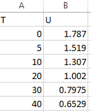
Dynamic viscosity of water
| T | 0 | 5 | 10 | 20 | 30 | 40 |
|
|
1.787 | 1.519 | 1.307 | 1.002 | 0.7975 | 0.6529 |
(a) Plot these data.
(b) Use interpolation to predict
(c) Use polynomial regression to fit a parabola to these data in order to make the same prediction.
(a)
To graph: The given data if
| T | 0 | 5 | 10 | 20 | 30 | 40 |
| 1.787 | 1.519 | 1.307 | 1.002 | 0.7975 | 0.6529 |
Explanation of Solution
Given Information:
The data is,
| T | 0 | 5 | 10 | 20 | 30 | 40 |
| 1.787 | 1.519 | 1.307 | 1.002 | 0.7975 | 0.6529 |
Graph:
The plot can be easily made with the help of excel as shown below,
Step 1. First put the data in the excel as shown below,
Step 2. Now click on insert and then scatter plot.
Thus, the scatter plot is,
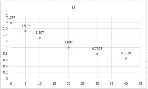
Interpretation:
From the plot, this can be interpreted that the dynamic viscosity of water decreases as the temperature increases.
(b)
To calculate: The value of
| T | 0 | 5 | 10 | 20 | 30 | 40 |
| 1.787 | 1.519 | 1.307 | 1.002 | 0.7975 | 0.6529 |
Answer to Problem 48P
Solution:
The value of
Explanation of Solution
Given Information:
The data is,
| T | 0 | 5 | 10 | 20 | 30 | 40 |
| 1.787 | 1.519 | 1.307 | 1.002 | 0.7975 | 0.6529 |
Formula used:
The zero-order Newton’s interpolation formula:
The first-order Newton’s interpolation formula:
The second- order Newton’s interpolating polynomial is given by,
The n th-order Newton’s interpolating polynomial is given by,
Where,
The first finite divided difference is,
And, the n th finite divided difference is,
Calculation:
To solve for
Assume
First, order the provided value as close to 7.5 as below,
Therefore,
And,
The first divided difference is,
Thus, the first degree polynomial value can be calculated as,
Put
Solve for other values as,
And,
Similarly,
The second divided difference is,
Thus, the second degree polynomial value can be calculated as,
Put
And,
The third divided difference is,
Thus, the third degree polynomial value can be calculated as,
Put this in above equation,
Therefore,
And, the error is calculated as,
Similarly the other dividend can be calculated as shown above,
Therefore, the difference table can be summarized for
| Order | Error | |
| 0 | ||
| 1 | ||
| 2 | ||
| 3 | ||
| 4 | ||
| 5 |
Since the minimum error for order four, therefore, it can be concluded that the value of
(c)
To calculate: The value of
| T | 0 | 5 | 10 | 20 | 30 | 40 |
| 1.787 | 1.519 | 1.307 | 1.002 | 0.7975 | 0.6529 |
Answer to Problem 48P
Solution:
The value of
Explanation of Solution
Given Information:
The data is,
| T | 0 | 5 | 10 | 20 | 30 | 40 |
| 1.787 | 1.519 | 1.307 | 1.002 | 0.7975 | 0.6529 |
Calculation:
This problem can be easily solved with the help of excel as shown below,
Step 1. First put the data in the excel as shown below,
Step 2. Now click on insert and then scatter plot.
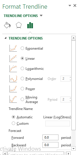
Step 3. Click on layout, Trendline, more trendline options, polynomial and then display equation on chart.
Step 4. Click on display R-squared value on chart as shown below,
Thus, the final plot is shown as below,
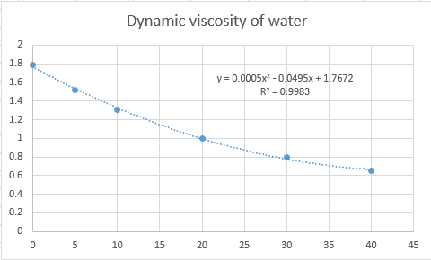
Therefore, the regression plot equation of the data will be,
Put
Hence, the value of
Want to see more full solutions like this?
Chapter 20 Solutions
Numerical Methods for Engineers


- The population Pinmillions of Texas from 2001 through 2014 can be approximated by the model P=20.913e0.0184t, where t represents the year, with t=1 corresponding to 2001. According to this model, when will the population reach 32 million?arrow_forwardA Dubious Model of Oil Prices The following table shows the prices of oil in U.S. dollars per barrel, t years since 1990, One analysis involving additional data used a cubic equation to model this data. t Years since 1990 0 2 5 7 10 12 15 17 20 21 P Price, dollars per barrel 18.91 16.22 16.63 18.20 27.04 23.47 49.63 69.04 77.46 106.92 a. Use cubic regression to model these data. Round the regression parameters to four decimal places. b. Plot the data along with the cubic model. c. In the analysis mentioned above, the graph is expanded through 2020. Expand the viewing window to show the model from 1990 to 2020. d. What estimate does the model give for oil prices in 2015? e. The actual price of oil in December of 2015 was about 35 per barrel. What basic principle in the use of models would be violated in relying on the estimate in part d?arrow_forwardThe following fictitious table shows kryptonite price, in dollar per gram, t years after 2006. t= Years since 2006 0 1 2 3 4 5 6 7 8 9 10 K= Price 56 51 50 55 58 52 45 43 44 48 51 Make a quartic model of these data. Round the regression parameters to two decimal places.arrow_forward
 Functions and Change: A Modeling Approach to Coll...AlgebraISBN:9781337111348Author:Bruce Crauder, Benny Evans, Alan NoellPublisher:Cengage Learning
 Trigonometry (MindTap Course List)TrigonometryISBN:9781337278461Author:Ron LarsonPublisher:Cengage Learning
 Linear Algebra: A Modern IntroductionAlgebraISBN:9781285463247Author:David PoolePublisher:Cengage Learning
 Algebra & Trigonometry with Analytic GeometryAlgebraISBN:9781133382119Author:SwokowskiPublisher:Cengage