Numerical Methods for Engineers
7th Edition
ISBN: 9780073397924
Author: Steven C. Chapra Dr., Raymond P. Canale
Publisher: McGraw-Hill Education
bartleby

Concept explainers

bartleby

Videos

Textbook Question
Book Icon
Chapter 20, Problem 16P

Soft tissue follows an exponential deformation behavior in uniaxial tension while it is in the physiologic or normal range of elongation. This can be expressed as

σ = E 0 a ( e a ε 1 )

where σ = stress, ε = strain, and E 0 anda are material constants that are determined experimentally. To evaluate the two material constants, the above equation is differentiated with respect to ε . Using the above equation establishes the fundamental relationship for soft tissue

d σ d ε = E 0 + a σ

To evaluate E 0 and a, stress-strain data are plotted as d σ / d ε versus σ and the intercept and slope of this plot are the two material constants, respectively.

In the following table is stress-strain data for heart chordate tendineae (small tendons used to hold heart valves closed during contraction of the heart muscle; these data are from loading the tissue, while different curves are produced on unloading).

σ ,   1 0 3 N/m 2 87.8 96.6 176 263 351 571 834 1229 1624 2107 2678 3380 4258
ε ,  10 3 m/m 153 204 255 306 357 408 459 510 561 612 663 714 765

Calculate the derivative d σ / d ε using finite differences. Plot these data and eliminate the data points near the zero points that appear not to follow the straight-line relationship. The error in these data comes from the inability of the instrumentation to read the small values in this region. Perform a regression analysis of the remaining data points to determine the values of E 0 and a.

Plot the stress versus strain data points along with the analytic curve expressed by the first equation. This will indicate how well the analytic curve matches these data.

Many times this does not work well because the value of E 0 is difficult to evaluate using this technique. To solve this problem E 0 is not used. A data point is selected ( σ ¯ , ε ¯ ) that is in the middle of the regression analysis range. These values are substituted into the first equation and a value for E 0 / a is determined and substituted into the first equation, which becomes

σ = ( σ ¯ e a ε ¯ 1 ) ( e a ε 1 )

Using this approach, experimental data that are well defined will produce a good match of the data points and the analytic curve. Use this new relationship and again plot the stress versus strain data points and this new analytic curve.

Expert Solution & Answer
Check Mark
To determine

To calculate: The values of E0 and a using a regression analysis on the derivatives based on finite differences of the provided data points and then obtain a function of the form σ=E0a(eaε1) that fits the data points correctly.

Answer to Problem 16P

Solution: The function that fits the data perfectly is σ=804.5591945812(e0.0035499643ε1).

Explanation of Solution

Given Information:

The provided values of the stress σ in 103N/m2 based on the strain ε in 103m/m are:

σ, 103N/m2 87.8 96.6 176 263 351 571
ε, 103m/m 153 204 255 306 357 408

And,

σ, 103N/m2 834 1229 1624 2107 2678 3380 4258
ε, 103m/m 459 510 561 612 663 714 765

Formula Used:

The formula for the derivative of a function at a point c using forward difference is:

f'(c)=f(c+h)f(c)h

The formula for the derivative of a function at a point c using backward difference is:

f'(c)=f(c)f(ch)h

The formula for the derivative of a function at a point c using central difference is:

f'(c)=f(c+h)f(ch)2h

Calculation:

Consider the formula for the stress:

σ=E0a(eaε1)

Differentiate both sides with respect to ε to obtain:

dσdε=E0+aσ

This is a linear equation.

First obtain the value of the derivative of the stress σ at the first data point using the forward difference. Note that the data is equally spaced with a step-size of 51.

σ'(153)=ε(204)ε(153)51=96.687.851=0.1725

Now the derivative at the second data point can be obtained using the central difference. Note that the data is equally spaced with a step-size of 51.

σ'(204)=ε(255)ε(153)51=17687.82(51)=0.8647

Now do the same for all the data points except the last one:

σ'(255)=26396.62(51)=1.6314σ'(306)=3511762(51)=1.7157

And,

σ'(357)=5712632(51)=3.0196σ'(408)=8343512(51)=4.7353

And,

σ'(459)=12295712(51)=6.4510σ'(510)=16248342(51)=7.7451

And,

σ'(561)=210712292(51)=8.6078σ'(612)=267816242(51)=10.3333

And,

σ'(663)=338021072(51)=12.4804σ'(714)=425826782(51)=15.4902

Now the derivative at the last data point can be obtained using the backward difference. Note that the data is equally spaced with a step-size of 51.

σ'(153)=ε(765)ε(714)51=4258338051=17.2157

Hence, the derivatives have been obtained as:

σεσ'(ε)87.81530.172596.62040.86471762551.63142633061.71573513573.01965714084.73538344596.451012295107.745116245618.6078210761210.3333267866312.4804338071415.4902425876517.2157

Now perform a regression analysis on the derivative with respect to σ and obtain a linear equation for the derivative in terms of σ.

This can be done using MS-Excel.

Step 1: Enter the data points in a blank workbook.

Step 2: Select the data points, go to insert and the select scatter plot.

This gives:

Numerical Methods for Engineers, Chapter 20, Problem 16P , additional homework tip  1

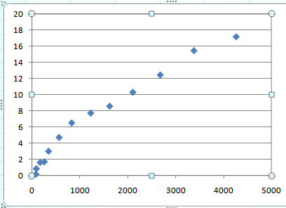
It can be seen that the first four points do not follow a linear relationship. So disregard the first four points and obtain a line of best fit for the remaining points.

This can be done using MATLAB.

Code:

clc;

clear all;

% Enter the data points

Stress=[87.896.6176263351571834122916242107267833804258];

Strain=153:51:765;

% Enter the derivative values calculated

Diff=[0.17250.86471.63141.71573.01964.73536.5417.74518.607810.333312.480415.490217.2157];

% Select the new data excluding the first four data points

Newdata=[Stress(5:end);Diff(5:end)];

% Perform a linear regression on these points

polyfit(Newdata(1, :),Newdata(2, :),1);

Output:

Numerical Methods for Engineers, Chapter 20, Problem 16P , additional homework tip  2

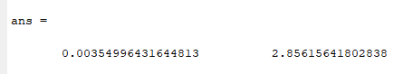
This implies that the linear model for the derivative is:

dσdε=2.8561564180+0.0035499643σ

This gives the value of a as 0.0035499643 and the value of E0 as 2.8561564180.

Now, substitute this in the formula for stress to obtain:

σ=2.85615641800.0035499643(e0.0035499643ε1)=804.5591945812(e0.0035499643ε1)

To check whether this model is a good fit for the data, plot this model along with the provided data points. This can be done using MATLAB.

Code:

clc;

clear all;

% Enter the data points

Stress=[87.896.6176263351571834122916242107267833804258];

Strain=153:51:765;

% Enter the derivative values calculated

Diff=[0.17250.86471.63141.71573.01964.73536.5417.74518.607810.333312.480415.490217.2157];

% Select the new data excluding the first four data points

Newdata=[Stress(5:end);Diff(5:end)];

% Perform a linear regression on these points

polyfit(Newdata(1, :),Newdata(2, :),1);

% Enter the formula for Stress obtained using the values of E0 and a

eqn=804.5591945812*(exp(0.0035499643*Strain)-1);

% Now plot the points along with the data

scatter(Strain,Stress);hold on

plot(Strain,eqn)

Output:

Numerical Methods for Engineers, Chapter 20, Problem 16P , additional homework tip  3

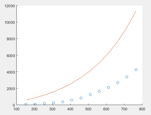
Clearly, the obtained function is not a good fit for the data.

Rewrite the expression for the original functionto obtain:

E0a=σ(eaε1)

Use this to obtain:

σ=σ'eaε'1(eaε1)

Now consider a data point in the middle of the data (σ',ε')=(2107,612).

Use this to get the formula for the strain as:

σ=2107e0.0035499643(612)1(e0.0035499643ε1)=2107e0.0035499643(612)1(e0.0035499643ε1)=270.79152781(e0.0035499643ε1)

To check whether this model is a good fit for the data, plot this model along with the provided data points. This can be done using MATLAB.

Code:

clc;

clear all;

% Enter the data points

Stress=[87.896.6176263351571834122916242107267833804258];

Strain=153:51:765;

% Enter the derivative values calculated

Diff=[0.17250.86471.63141.71573.01964.73536.5417.74518.607810.333312.480415.490217.2157];

% Select the new data excluding the first four data points

Newdata=[Stress(5:end);Diff(5:end)];

% Perform a linear regression on these points

polyfit(Newdata(1, :),Newdata(2, :),1);

% Enter the formula for Stress obtained using the values of E0 and a

eqn=804.5591945812*(exp(0.0035499643*Strain)-1);

eqn_new=270.79152781*(exp(0.0035499643*Strain)-1);

% Now plot the points along with the data

scatter(Strain,Stress);hold on

plot(Strain,eqn_new)

Output:

Numerical Methods for Engineers, Chapter 20, Problem 16P , additional homework tip  4

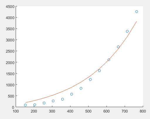
It is clear that the function obtained using the data point from the middle is a much better fit for the provided data points.

Hence, the desired function that fits the data points is σ=804.5591945812(e0.0035499643ε1).

Want to see more full solutions like this?

Subscribe now to access step-by-step solutions to millions of textbook problems written by subject matter experts!

Chapter 20 Solutions

Numerical Methods for Engineers

Ch. 20 - Prob. 11PCh. 20 - The molecular weight of a polymer can be...Ch. 20 - 20.13 On average, the surface area A of human...Ch. 20 - 20.14 Determine an equation to predict metabolism...Ch. 20 - 20.15 Human blood behaves as a Newtonian fluid...Ch. 20 - 20.16 Soft tissue follows an exponential...Ch. 20 - 20.17 The thickness of the retina changes during...Ch. 20 - 20.18 The data tabulated below were generated from...Ch. 20 - The shear stresses, in kilopascals (kPa), of nine...Ch. 20 - 20.20 A transportation engineering study was...Ch. 20 - The saturation concentration of dissolved oxygen...Ch. 20 - For the data in Table P20.21, use polynomial...Ch. 20 - 20.23 Use multiple linear regression to derive a...Ch. 20 - 20.24 As compared to the models from Probs. 20.22...Ch. 20 - 20.25 In water-resources engineering, the sizing...Ch. 20 - 20.26 The concentration of total phosphorus and...Ch. 20 - 20.27 The vertical stress under the corner of a...Ch. 20 - Three disease-carrying organisms decay...Ch. 20 - 20.29 The mast of a sailboat has a cross-sectional...Ch. 20 - 20.30 Enzymatic reactions are used extensively to...Ch. 20 - 20.31 Environmental engineers dealing with the...Ch. 20 - An environmental engineer has reported the data...Ch. 20 - The following model is frequently used in...Ch. 20 - 20.34 As a member of Engineers Without Borders,...Ch. 20 - 20.35 Perform the same computations as in Sec....Ch. 20 - 20.36 You measure the voltage drop V across a...Ch. 20 - Duplicate the computation for Prob. 20.36, but use...Ch. 20 - The current in a wire is measured with great...Ch. 20 - 20.39 The following data was taken from an...Ch. 20 - It is known that the voltage drop across an...Ch. 20 - Ohms law states that the voltage drop V across an...Ch. 20 - 20.42 Repeat Prob. 20.41 but determine the...Ch. 20 - 20.43 An experiment is performed to determine the...Ch. 20 - Bessel functions often arise in advanced...Ch. 20 - 20.45 The population of a small community on the...Ch. 20 - Based on Table 20.4, use linear and quadratic...Ch. 20 - 20.47 Reproduce Sec. 20.4, but develop an equation...Ch. 20 - 20.48 Dynamic viscosity of water is related to...Ch. 20 - 20.49 Hooke’s law, which holds when a spring is...Ch. 20 - 20.50 Repeat Prob. 20.49 but fit a power curve to...Ch. 20 - The distance required to stop an automobile...Ch. 20 - An experiment is performed to define the...Ch. 20 - The acceleration due to gravity at an altitude y...Ch. 20 - The creep rate is the time rate at which strain...Ch. 20 - 20.55 It is a common practice when examining a...Ch. 20 - The relationship between stress and the shear...Ch. 20 - The velocity u of air flowing past a flat surface...Ch. 20 - 20.58 Andrade’s equation has been proposed as a...Ch. 20 - Develop equations to fit the ideal specific heats...Ch. 20 - 20.60 Temperatures are measured at various points...Ch. 20 - 20.61 The data below were obtained from a creep...
Knowledge Booster
Background pattern image
Advanced Math
Learn more about
Need a deep-dive on the concept behind this application? Look no further. Learn more about this topic, advanced-math and related others by exploring similar questions and additional content below.
Recommended textbooks for you
Text book image
Advanced Engineering Mathematics
Advanced Math
ISBN:9780470458365
Author:Erwin Kreyszig
Publisher:Wiley, John & Sons, Incorporated
Text book image
Numerical Methods for Engineers
Advanced Math
ISBN:9780073397924
Author:Steven C. Chapra Dr., Raymond P. Canale
Publisher:McGraw-Hill Education
Text book image
Introductory Mathematics for Engineering Applicat...
Advanced Math
ISBN:9781118141809
Author:Nathan Klingbeil
Publisher:WILEY
Text book image
Mathematics For Machine Technology
Advanced Math
ISBN:9781337798310
Author:Peterson, John.
Publisher:Cengage Learning,
Text book image
Basic Technical Mathematics
Advanced Math
ISBN:9780134437705
Author:Washington
Publisher:PEARSON
Text book image
Topology
Advanced Math
ISBN:9780134689517
Author:Munkres, James R.
Publisher:Pearson,
01 - What Is A Differential Equation in Calculus? Learn to Solve Ordinary Differential Equations.; Author: Math and Science;https://www.youtube.com/watch?v=K80YEHQpx9g;License: Standard YouTube License, CC-BY
Higher Order Differential Equation with constant coefficient (GATE) (Part 1) l GATE 2018; Author: GATE Lectures by Dishank;https://www.youtube.com/watch?v=ODxP7BbqAjA;License: Standard YouTube License, CC-BY
Solution of Differential Equations and Initial Value Problems; Author: Jefril Amboy;https://www.youtube.com/watch?v=Q68sk7XS-dc;License: Standard YouTube License, CC-BY