
Videos
a.
Calculate the class width for the data on depths below surface grade at which significant artifacts were discovered.
a.
Answer to Problem 18P
The class width is calculated as 28.
Explanation of Solution
Calculation:
From the given data set, the largest data point is 200 and the smallest data point is 10.
Class Width:
The class width is calculated as follows:
b.
Create a table for frequency distribution with class limits, class boundaries, midpoints, frequencies, relative frequencies, and cumulative frequencies.
b.
Answer to Problem 18P
The class limits for a frequency table with 7 classes using class width 28 are 10-37, 38-65, 66-93, 94-121, 122-149, 150-177, and 178-205.
Explanation of Solution
Class limits:
Class limits are the maximum and minimum values in the class interval
Class Boundaries:
A class boundary is the midpoint between the upper limit of one class and the lower limit of the next class where the upper limit of the preceding class interval and the lower limit of the next class interval will be equal. The upper class boundary is calculated by adding 0.5 to the upper class limit and the lower class boundary is calculated by subtracting 0.5 from the lower class limit.
Midpoint:
The midpoint is calculated as given below:
Frequency:
Frequency is the number of data points that fall under each class.
Cumulative frequency:
Cumulative frequency is calculated by adding each frequency to the sum of preceding frequencies.
Relative Frequency:
Relative frequency is the ratio of frequency by the total number of data values.
The class width is 28. Hence, the lower class limit for the second class 261 is calculated by adding 25 to 236. Following this pattern, all the lower class limits are established. Then, the upper class limits are calculated.
The frequency distribution table is given below:
| Class Limits | Class Boundaries | Midpoints | Frequency | Relative Frequency | Cumulative Frequency |
| 10-37 | 9.5-37.5 |
23.5 | 7 | 7 | |
| 38-65 | 37.5-65.5 | 51.5 | 25 | 32 (=25+7) | |
| 66-93 | 65.5-93.5 | 79.5 | 26 | 58 (=26+32) | |
| 94-121 | 93.5-121.5 | 107.5 | 9 | 67 (=9+58) | |
| 122-149 | 121.5-149.5 | 135.5 | 5 | 72 (=5+67) | |
| 150-177 | 149.5-177.5 | 163.5 | 0 | 72 (=0+72) | |
| 178-205 | 177.5-205.5 | 191.5 | 1 | 73 (=1+72) |
c.
Create a histogram for the given data on depths below surface grade at which significant artifacts were discovered.
c.
Answer to Problem 18P
The frequency histogram for the data on depths below surface grade at which significant artifacts were discovered is shown below:
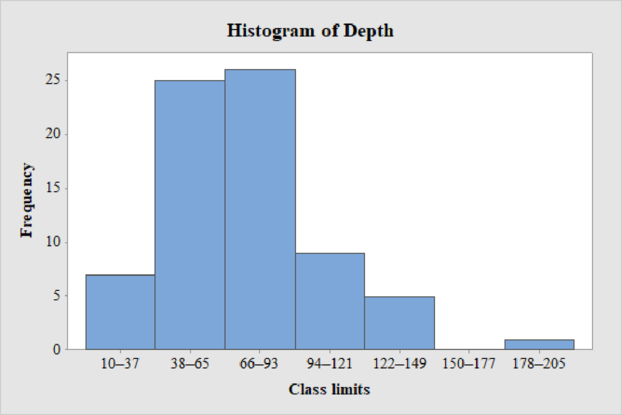
Explanation of Solution
Step-by-step procedure to draw the histogram using MINITAB software:
- Choose Graph > Bar Chart.
- From Bars represent, choose Values from a table.
- Under One column of values, choose Simple. Click OK.
- In Graph variables, enter the column of Frequency.
- In Categorical variable, enter the column of Class Limits.
- Click OK.
Thus, the histogram for depth is obtained.
d.
Construct a relative frequency histogram for the data on depths below surface grade at which significant artifacts were discovered.
d.
Answer to Problem 18P
The relative frequency histogram for the data on depths below surface grade at which significant artifacts were discovered is shown below:
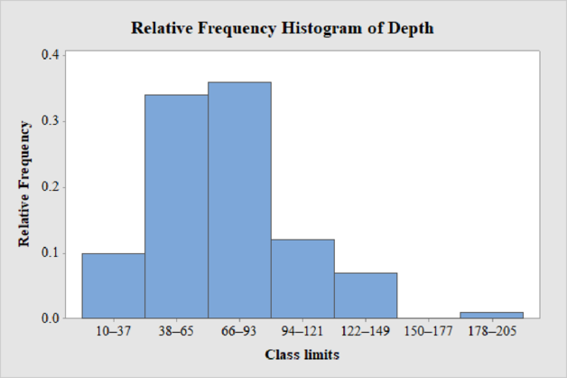
Explanation of Solution
Step-by-step procedure to draw the histogram using MINITAB software:
- Choose Graph > Bar Chart.
- From Bars represent, choose Values from a table.
- Under One column of values, choose Simple. Click OK.
- In Graph variables, enter the column of Relative Frequency Class Limits.
- In Categorical variable, enter the column of Class Limits.
- Click OK.
Thus, the relative frequency histogram for depth is obtained.
e.
Identify the shape of distribution: uniform, mound shaped, symmetric, bimodal, skewed left, or skewed right.
e.
Explanation of Solution
From the histogram, the distribution of depths below surface grade at which significant artifacts were discovered is right-skewed and there is an unusual observation in the data.
f.
Create an ogive curve for the given data on depths below surface grade at which significant artifacts were discovered.
f.
Answer to Problem 18P
An ogive curve for the depths below surface grade at which significant artifacts were discovered is shown below:
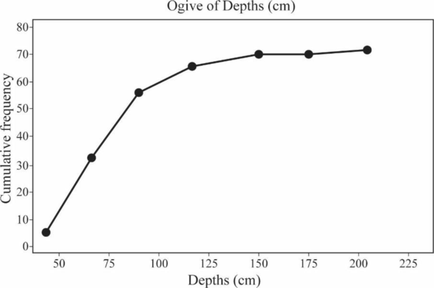
Explanation of Solution
Step-by-step procedure to draw the Ogive curve:
- Draw X axis with data values ranging from 50 to 225.
- Label the X axis as Depths (cm).
- Draw Y axis with data values Cumulative frequency ranging from.0 to 80.
- Label the Y axis as Cumulative frequency.
- Plot the cumulative frequencies
- Join the points and draw an ogive curve.
Thus, an ogive curve for depth is obtained.
g.
Identify the characteristics about the depths below surface grade at which significant artifacts were discovered using the graphs.
g.
Explanation of Solution
The data values of depths below surface grade fall within 10 and 200.
The
The central value of the data is approximately 65.5.
From the histogram, it can be observed that the data is right-skewed and the outlier is 200.
Want to see more full solutions like this?
Chapter 2 Solutions
Understandable Statistics: Concepts and Methods


 Holt Mcdougal Larson Pre-algebra: Student Edition...AlgebraISBN:9780547587776Author:HOLT MCDOUGALPublisher:HOLT MCDOUGAL