
Videos
a.
Construct the frequency distribution with approximately 5classes.
a.
Answer to Problem 31E
The frequency distribution is,
| Number of Words | Frequency |
| 0-1,999 | 26 |
| 2,000-3,999 | 25 |
| 4,000-5,999 | 5 |
| 6,000-7,999 | 0 |
| 8,000-9,999 | 1 |
| Total | 57 |
Explanation of Solution
Calculation:
The given information is that a table representing the number of words spoken in each of these addresses.
Frequency:
The frequencies are calculated by using the tally mark and the
- Based on the given information, the class intervals are 0-1,999, 2,000-3,999, 4,000-5,999, 6,000-7,999, 8,000-9,999.
- Make a tally mark for each value in the corresponding number of words spoken and continue for all values in the data.
- The number of tally marks in each class represents the frequency, f of that class.
Similarly, the frequency of remaining classes for the number of words spoken is given below:
| Number of Words | Tally | Frequency |
| 0-1,999 | 26 | |
| 2,000-3,999 | 25 | |
| 4,000-5,999 | 5 | |
| 6,000-7,999 | 0 | |
| 8,000-9,999 | 1 | |
| Total | 57 |
b.
Construct the frequency histogram based on the frequency distribution.
b.
Answer to Problem 31E
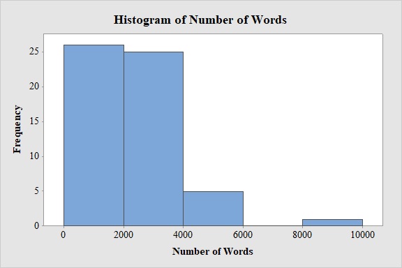
Output obtained from MINITAB software for the number of words spoken is:
Explanation of Solution
Calculation:
Frequency Histogram:
Software procedure:
- Step by step procedure to draw the relative frequency histogram for number of words spoken using MINITAB software.
- Choose Graph > Histogram.
- Choose Simple.
- Click OK.
- In Graph variables, enter the column of Number of Words.
- In Scale, Choose Y-scale Type as Frequency.
- Click OK.
- Select Edit Scale, Enter 0, 2,000, 4,000, 6,000, 8,000, 10,000 in Positions of ticks.
- In Binning, Under Interval Type select Cutpoint and under Interval Definition select Number of intervals as 5 and Cutpoint positions as 0, 2,000, 4,000, 6,000, 8,000, 10,000.
- In Labels, Enter 0, 2,000, 4,000, 6,000, 8,000, 10,000 in Specified.
- Click OK.
Observation:
From the bar graph, it can be seen that maximum number of words spoken are in the interval 0-2,000.
c.
Construct a relative frequency distribution for the data.
c.
Answer to Problem 31E
The relative frequency distribution for the data is:
| Number of Words | Relative frequency |
| 0-1,999 | 0.456 |
| 2,000-3,999 | 0.439 |
| 4,000-5,999 | 0.088 |
| 6,000-7,999 | 0.000 |
| 8,000-9,999 | 0.018 |
Explanation of Solution
Calculation:
Relative frequency:
The general formula for the relative frequency is,
Therefore,
Similarly, the relative frequencies for the remaining number of words spoken are obtained below:
| Number of Words | Frequency | Relative frequency |
| 0-1,999 | 26 | |
| 2,000-3,999 | 25 | |
| 4,000-5,999 | 5 | |
| 6,000-7,999 | 0 | |
| 8,000-9,999 | 1 |
d.
Construct the relative frequency histogram based on the frequency distribution.
d.
Answer to Problem 31E
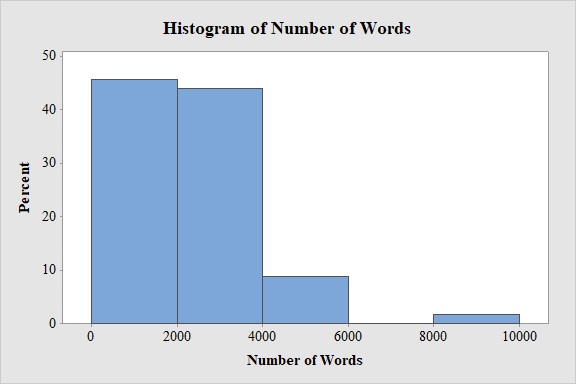
Output obtained from MINITAB software for the number of words spoken is:
Explanation of Solution
Calculation:
Relative Frequency Histogram:
Software procedure:
- Step by step procedure to draw the relative frequency histogram for the number of words spoken using MINITAB software.
- Choose Graph > Histogram.
- Choose Simple.
- Click OK.
- In Graph variables, enter the column of Number of Words.
- In Scale, Choose Y-scale Type as Percent.
- Click OK.
- Select Edit Scale, Enter 0, 2,000, 4,000, 6,000, 8,000, 10,000 in Positions of ticks.
- In Binning, Under Interval Type select Cutpoint and under Interval Definition select Number of intervals as 5 and Cutpoint positions as 0, 2,000, 4,000, 6,000, 8,000, 10,000.
- In Labels, Enter 0, 2,000, 4,000, 6,000, 8,000, 10,000 in Specified.
- Click OK.
Observation:
From the bar graph, it can be seen that maximum number of words spoken is in the interval 0-2,000.
e.
Check whether the histograms are skewed to the left, skewed to the right or approximately symmetric.
e.
Answer to Problem 31E
The histogram is skewed to the right.
Explanation of Solution
From the given histogram, the right hand tail is larger than the left hand tail from the maximum frequency value. Hence, the shape of the distribution is right skewed.
f.
Construct the frequency distribution with approximately 9classes.
f.
Answer to Problem 31E
The frequency distribution is,
| Number of Words | Frequency |
| 0-999 | 4 |
| 1,000-1,999 | 22 |
| 2,000-2,999 | 18 |
| 3,000-3,999 | 7 |
| 4,000-4,999 | 4 |
| 5,000-5,999 | 1 |
| 6,000-6,999 | 0 |
| 7,000-7,999 | 0 |
| 8,000-8,999 | 1 |
| Total | 57 |
Explanation of Solution
Calculation:
Frequency:
The frequencies are calculated by using the tally mark and the range of the data is from 0 to 8,999.
- Based on the given information, the class intervals are 0-999, 1,000-1,999, 2,000-2,999, 3,000-3,999, 4,000-4,999, 5,000-5,999, 6,000-6,999, 7,000-7,999, 8,000-8,999.
- Make a tally mark for each value in the corresponding number of words spoken and continue for all values in the data.
- The number of tally marks in each class represents the frequency, f of that class.
Similarly, the frequency of remaining classes for the number of words spoken is given below:
| Number of Words | Tally | Frequency |
| 0-999 | 4 | |
| 1,000-1,999 | 22 | |
| 2,000-2,999 | 18 | |
| 3,000-3,999 | 7 | |
| 4,000-4,999 | 4 | |
| 5,000-5,999 | 1 | |
| 6,000-6,999 | 0 | |
| 7,000-7,999 | 0 | |
| 8,000-8,999 | 1 | |
| Total | 57 |
g.
Repeat parts (b) to (d), using the frequency distribution constructed in part (f).
g.
Answer to Problem 31E
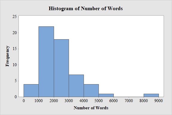
Output obtained from MINITAB software for the number of words spoken is:
The relative frequency distribution for the data is:
| Number of Words | Relative frequency |
| 0-999 | 0.070 |
| 1,000-1,999 | 0.386 |
| 2,000-2,999 | 0.316 |
| 3,000-3,999 | 0.123 |
| 4,000-4,999 | 0.070 |
| 5,000-5,999 | 0.018 |
| 6,000-6,999 | 0.000 |
| 7,000-7,999 | 0.000 |
| 8,000-8,999 | 0.018 |
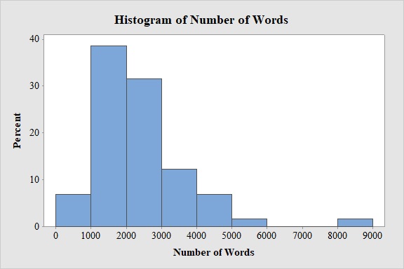
Output obtained from MINITAB software for the number of words spoken is:
Explanation of Solution
Calculation:
Frequency Histogram:
Software procedure:
- Step by step procedure to draw the relative frequency histogram for the number of words spoken using MINITAB software.
- Choose Graph > Histogram.
- Choose Simple.
- Click OK.
- In Graph variables, enter the column of Number of Words.
- In Scale, Choose Y-scale Type as Frequency.
- Click OK.
- Select Edit Scale, Enter 0, 1,000, 2,000, 3,000, 4,000, 5,000, 6,000, 7,000, 8,000, 90,00 in Positions of ticks.
- In Binning, Under Interval Type select Cutpoint and under Interval Definition select Number of intervals as 9 and Cutpoint positions as 0, 1,000, 2,000, 3,000, 4,000, 5,000, 6,000, 7,000, 8,000, 9,000.
- In Labels, Enter 0, 1,000, 2,000, 3,000, 4,000, 5,000, 6,000, 7,000, 8,000, 9,000 in Specified.
- Click OK.
Observation:
From the bar graph, it can be seen that maximum number of words spoken is in the interval 1,000-2,000.
Relative frequency:
Similarly, the relative frequencies for the remaining number of words spoken are obtained below:
| Number of Words | Frequency | Relative frequency |
| 0-999 | 4 | |
| 1,000-1,999 | 22 | |
| 2,000-2,999 | 18 | |
| 3,000-3,999 | 7 | |
| 4,000-4,999 | 4 | |
| 5,000-5,999 | 1 | |
| 6,000-6,999 | 0 | |
| 7,000-7,999 | 0 | |
| 8,000-8,999 | 1 | |
| Total | 57 |
Relative Frequency Histogram:
Software procedure:
- Step by step procedure to draw the relative frequency histogram for the number of words spoken using MINITAB software.
- Choose Graph > Histogram.
- Choose Simple.
- Click OK.
- In Graph variables, enter the column of Number of Words.
- In Scale, Choose Y-scale Type as Percent.
- Click OK.
- Select Edit Scale, Enter 0, 1,000, 2,000, 3,000, 4,000, 5,000, 6,000, 7,000, 8,000 and 9,000 in Positions of ticks.
- In Binning, Under Interval Type select Cutpoint and under Interval Definition select Number of intervals as 9 and Cutpoint positions as 0, 1,000, 2,000, 3,000, 4,000, 5,000, 6,000, 7,000, 8,000 and 9,000.
- In Labels, Enter 0, 1,000, 2,000, 3,000, 4,000, 5,000, 6,000, 7,000, 8,000 and 9,000in Specified.
- Click OK.
Observation:
From the bar graph, it can be seen that maximum number of words spoken is in the interval 1,000-2,000.
h.
Check whether the 9 and 5 classes are reasonable or one choice is much better than the other and explain the reason.
h.
Answer to Problem 31E
Both the 5 and 9 classes are reasonable.
Explanation of Solution
Answer will vary.
The number of classes can be obtained by the following two points:
- The number of classes should be between 5 and 20.
- A larger number of classes will be appropriate for a very large data set.
Here number of classes for the histograms are 5 and 9 respectively. Thus, the number of classes are lies between 5 and 20.
Hence, the both 5 and 9 classes are reasonable.
Want to see more full solutions like this?
Chapter 2 Solutions
ESSENTIAL STATISTICS(FD)


 Glencoe Algebra 1, Student Edition, 9780079039897...AlgebraISBN:9780079039897Author:CarterPublisher:McGraw Hill