
a)
To construct a
a)
Explanation of Solution
Given:
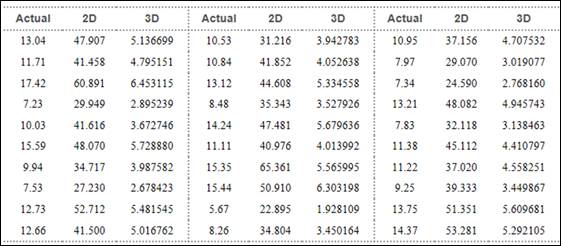
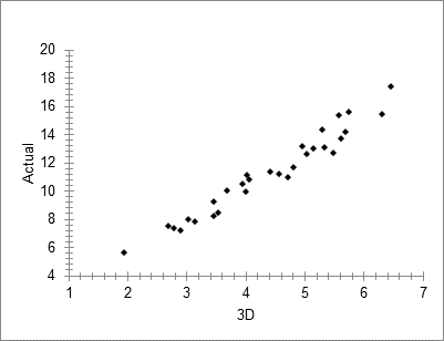
Scatter plot for Actual vs 3D volume construction is,
| r² | 0.954 | n | 30 | ||||
| r | 0.977 | k | 1 | ||||
| Std. Error | 0.649 | Dep. Var. | Actual | ||||
| ANOVA table | |||||||
| Source | SS | df | MS | F | p-value | ||
| Regression | 242.8360 | 1 | 242.8360 | 576.93 | 3.17E-20 | ||
| Residual | 11.7855 | 28 | 0.4209 | ||||
| Total | 254.6214 | 29 | |||||
| Regression output | confidence interval | ||||||
| variables | coefficients | std. error | t (df=28) | p-value | 95% lower | 95% upper | |
| Intercept | 0.4196 | 0.4671 | 0.898 | .3767 | -0.5373 | 1.3764 | |
| 3D | 2.4752 | 0.1031 | 24.019 | 3.17E-20 | 2.2641 | 2.6863 | |
Therefore, least square regression equation is,
b)
To verify the conditions for inference.
b)
Answer to Problem 23.30E
All the conditions satisfied.
Explanation of Solution
Given:
The scatter plot shows linearly increasing trend. Therefore, the relationship is clearly linear, the scatterplot shows no unusual pattern that would indicate not
c)
To test whether the linear relationship is statistically significant.
c)
Answer to Problem 23.30E
There is sufficient evidence to conclude that the linear relationship between two variables is statistically significant.
Explanation of Solution
Given:
| Regression Analysis | |||||||
| r² | 0.954 | n | 30 | ||||
| r | 0.977 | k | 1 | ||||
| Std. Error | 0.649 | Dep. Var. | Actual | ||||
| ANOVA table | |||||||
| Source | SS | df | MS | F | p-value | ||
| Regression | 242.8360 | 1 | 242.8360 | 576.93 | 3.17E-20 | ||
| Residual | 11.7855 | 28 | 0.4209 | ||||
| Total | 254.6214 | 29 | |||||
| Regression output | confidence interval | ||||||
| variables | coefficients | std. error | t (df=28) | p-value | 95% lower | 95% upper | |
| Intercept | 0.4196 | 0.4671 | 0.898 | .3767 | -0.5373 | 1.3764 | |
| 3D | 2.4752 | 0.1031 | 24.019 | 3.17E-20 | 2.2641 | 2.6863 | |
Null and alternative hypotheses:
Test statistic is,
t = 24.019
P-value = 0.0000
Decision: P-value< 0.05, reject H0.
Conclusion: There is sufficient evidence to conclude that the linear relationship between two variables is statistically significant.
Therefore, 95% confidence interval for slope is,
(2.2641, 2.6863)
Want to see more full solutions like this?
Chapter 23 Solutions
ACHIEVE F/PRACT OF STAT IN LIFE-ACCESS

 MATLAB: An Introduction with ApplicationsStatisticsISBN:9781119256830Author:Amos GilatPublisher:John Wiley & Sons Inc
 Probability and Statistics for Engineering and th...StatisticsISBN:9781305251809Author:Jay L. DevorePublisher:Cengage Learning
 Statistics for The Behavioral Sciences (MindTap C...StatisticsISBN:9781305504912Author:Frederick J Gravetter, Larry B. WallnauPublisher:Cengage Learning
 Elementary Statistics: Picturing the World (7th E...StatisticsISBN:9780134683416Author:Ron Larson, Betsy FarberPublisher:PEARSON
 The Basic Practice of StatisticsStatisticsISBN:9781319042578Author:David S. Moore, William I. Notz, Michael A. FlignerPublisher:W. H. Freeman
 Introduction to the Practice of StatisticsStatisticsISBN:9781319013387Author:David S. Moore, George P. McCabe, Bruce A. CraigPublisher:W. H. Freeman