Numerical Methods for Engineers
7th Edition
ISBN: 9789814670876
Author: Chapra
Publisher: BOOKXCHANG
bartleby

Videos

Textbook Question
Book Icon
Chapter 24, Problem 46P

The upward velocity of a rocket can be computed by the following formula:

v = u In ( m 0 m 0 q t ) g t

Where v = upword velocity, u = velocity at which fuel is expelled relative to the rocket, m 0 = initial mass of the rocket at time t = 0 ,

q = fuel consumption rate, and g = downword acceleration of gravity ( ( assumed constant = 9 .8 m/s 2 ) . If u = 1800 m/s , m 0 = 160 , 000 kg, and q = 2500 kg/s , use six-segment trapezoidal and Simpson's 1 / 3 rule, six-point Gauss quadrature, and O ( h 8 ) Romberg methods to determine how high the rocket will fly in 30 s. In addition, use numerical differentiation to generate a graph of acceleration as a function of time.

Expert Solution & Answer
Check Mark
To determine

To calculate: The height of the rocket at t=30sec using Six-segment trapezoidal, Simpson’s 1/3 rule, six-point Gauss quadrature and O(h8) Romberg methods. Also, generate a graph of acceleration as a function of time.

Answer to Problem 46P

Solution:

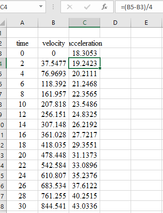
All the results are summarized in the table below,

1 2 3 4
n a 4.0634% 0.04927% 0.01159%
1 12668.115 10896.965 10875.5283 10880.57300
2 11339.7525 10880.8875 10879.31183
4 10995.60375 10879.70575
8 10908.68025

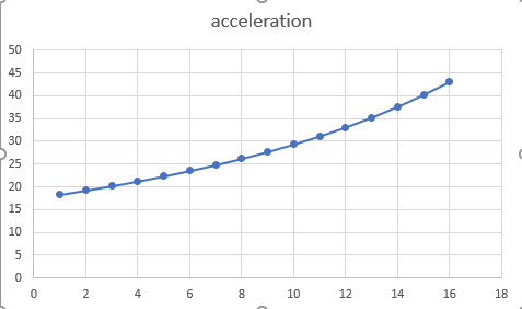
Acceleration graph is shown below.

Numerical Methods for Engineers, Chapter 24, Problem 46P , additional homework tip  1

Explanation of Solution

Given Information:

The formula for the upward velocity of rocket is given as,

v=uln(m0m0qt)gt

Here, v= upward velocity, u=1800 m/s Velocity at which fuel is expelled relative to the rocket

m0=160,000 kg Initial mass of the rocket at time t=a=0, q=2500 kg/s Fuel consumption rate, g=9.8m/s2, Downward acceleration of gravity, b=30 s is the final time.

Formula Used:

6-segment Trapezoidal rule.

I=ba2n[f(a)+2{i=1n1f(a+ih)}+f(b)]

6-segmentSimpson’s 1/3 rule.

I=ba3n[f(x0)+4iodd=1n1f(xi)+2ieven=2n2f(xi)+f(xn)]

Change of variable formula.

t=(b+a)+(ba)td2, dt=(ba)dtd2

Here, a and b are the lower and upper limits of the integral respectively.

Error Calculation.

a=|Actual value-Approx valueActual value|100%

Calculation:

Calculate the upward velocity of the rocket.

v=uln(m0m0qt)gt…… (1)

Substitute thegiven values in equation(1),

v=030(1800ln(160,000160,0002500t)9.8t)dt…… (2)

Apply 6-segment Trapezoidal rule for f(t)=v.

I=ba2n[f(a)+2{i=1n1f(a+ih)}+f(b)]

Here, h=ban

Substitute n=6, a=0 and b=30.

I=3002(6)[f(0)+2{i=15f(0+i(5))}+f(30)]

Expand the above terms.

I=3002(6)[f(0)+2{f(5)+f(10)+f(15)+f(20)+f(25)}+f(30)]…… (3)

Calculate f(0)

f(t)=1800ln(160,000160,0002500t)9.8t

Substitute t=0

f(0)=1800ln(160,000160,000(25000))(9.80)=0

Calculate f(5)

f(t)=1800ln(160,000160,0002500t)9.8t

Substitute t=5

f(5)=1800ln(160,000160,000(25005))(9.85)=97.4222

Calculate f(10)

f(t)=1800ln(160,000160,0002500t)9.8t

Substitute t=10

f(10)=1800ln(160,000160,000(250010))(9.810)=207.818

Similarly, calculate all the function values.

f(15)=333.713,f(20)=478.448f(25)=646.579,f(30)=844.541

Substitute above values in equation(3),

I=302(6)[0+2(97.4222+207.818+333.713+478.448+646.579)+844.541]=10931.2535

The formula for 6-segment Simpson’s 1/3 rule,

I=ba3n[f(x0)+4iodd=1n1f(xi)+2ieven=2n2f(xi)+f(xn)]

Substitute the function values from above,

I=3003(6)[f(0)+4{f(5)+f(15)+f(25)}+2{f(10)+f(20)}+f(30)]=303(6)[0+4{97.4222+333.713+646.579}+2{207.818+478.448}+844.541]=10879.883

The given velocity Integral is,

v=030(1800ln(160,000160,0002500t)9.8t)dt

Change of variable before integrating the function,

t=(b+a)+(ba)td2…… (4)

And

dt=(ba)dtd2…… (5)

Here, a and b are the lower and upper limits of the integral respectively.

Substitute the values of a=0 and b=30 in the equations(4) and (5),

t=15+15tddt=15dtd

Substitute the values of t and dt in equation(2),

v=030(1800ln(160,000160,0002500(15+15td))9.8(15+15td))15dtd

Thus, the transformed function is,

f(td)=(1800ln(160,000160,0002500(15+15td))9.8(15+15td))15

Apply Six-Point Gauss Quadrature formula.

I=0.1713245f(0.932469514)+0.3607616f(0.661209386)+0.4679139f(0.238619186)+0.4679139f(0.238619186)+0.3607616f(0.661209386)+0.1713245f(0.932469514)

Calculate f(0.932469514).

f(td)=(1800ln(160,000160,0002500(15+15td))9.8(15+15td))15

Substitute td=0.932469514.

f(0.932469514)=(1800ln(1600001600002500(15+15(0.932469514)))9.8(15+15(0.932469514)))(15)=281.855

Calculate f(0.661209386).

f(td)=(1800ln(160,000160,0002500(15+15td))9.8(15+15td))15

Substitute td=0.661209386.

f(0.661209386)=(1800ln(1600001600002500(15+15(0.661209386)))9.8(15+15(0.661209386)))(15)=1486.79

Similarly, calculate all function values.

f(0.238619186)=3628.30f(0.238619186)=6527.55f(0.661209386)=9654.10f(0.932469514)=12024.4

Substitute the values in Six-Point Gauss Quadrature formula.

I=0.1713245(281.855)+0.3607616(1486.79)+0.4679139(3628.30)+0.4679139(6527.55)+0.3607616(9654.10)+0.1713245(12024.4)=10879.63166

Apply Romberg Integration.

Choose h=30(distance between two consecutive ordinates), the values of v are,

t 0 30
v x0=0 x1=844.541

Substitute value from above and calculate I(h),

I(h)=h2(x0+x1)=302(0+844.541)=12668.115

Choose h=15, the values of v are,

t 0 15 30
v x0=0 x1=333.713 x2=844.541

Substitute values from above and calculate I(h2),

I(h2)=h2(x0+2x1+x2)=152(0+2(333.713)+844.541)=11339.7525

Choose h=7.5, the values of v are,

t 0 7.5 15 22.5 30
v x0=0 x1=150.856 x2=333.713 x3=559.241 x4=844.541

Substitute values from above and calculate I(h4),

I(h4)=h2(x0+2(x1+x2+x3)+x4)=7.52(0+2(150.856+333.713+559.241)+844.541)=10995.60375

Choose h=3.75, the values of v are,

t 0 3.75 7.5 11.25
v x0=0 x1=71.9349 x2=150.856 x3=237.725
15 18.75 22.5 26.25 30
x4=333.713 x5=440.275 x6=559.241 x7=692.966 x8=844.541

Substitute values from above and calculate I(h8),

I(h8)=h2(x0+2(x1+x2+x3+x4+x5+x6+x7)+x8)=3.752(0+2(71.9349+150.856+237.725+333.713+440.275+559.241+692.966)+844.541)=10908.68025

Substitute values from above and calculate I(h,h2),

I(h,h2)=13[4I(h2)I(h)]=13[4(11339.7525)12668.115]=10896.965

Calculate the approximate error,

a=|Actual value-Approx valueActual value|100%

Substitute values from above.

a=|10896.96511339.752510896.965|100%a=4.0634%

Substitute values from above and calculate I(h2,h4),

I(h2,h4)=13[4I(h4)I(h2)]=13[4(10995.60375)11339.7525]=10880.8875

Substitute values from above and calculate I(h4,h8),

I(h4,h8)=13[4I(h8)I(h4)]=13[4(10908.68025)10995.60375]=10879.70575

Substitute values from above and calculate I(h,h2,h4),

I(h,h2,h4)=13[4I(h2,h4)I(h,h2)]=13[4(10880.8875)10896.965]=10875.5283

Calculate the approximate error,

a=|Actual value-Approx valueActual value|100%

Substitute values from above,

a=|10875.528310880.887510875.5283|100%a=0.04927%

Substitute values from above and calculate I(h2,h4,h8),

I(h2,h4,h8)=13[4I(h4,h8)I(h2,h4)]=13[4(10879.70575)10880.8875]=10879.31183

Substitute values from above and calculate I(h,h2,h4,h8),

I(h,h2,h4,h8)=13[4I(h2,h4,h8)I(h,h2,h4)]=13[4(10879.31183)10875.5283]=10880.5730

Calculate the approximate error as,

a=|Actual value-Approx valueActual value|100%

Substitute values from above.

a=|10880.5730010879.3118310880.57300|100%a=0.01159%

All above calculated results are summarized in the table below,

1 2 3 4
n a 4.0634% 0.04927% 0.01159%
1 12668.115 10896.965 10875.5283 10880.57300
2 11339.7525 10880.8875 10879.31183
4 10995.60375 10879.70575
8 10908.68025

UseNumerical differentiation to calculate acceleration as a function of time.

Apply finite-divided differences for h=2,

a(0)=dv(0)dt=3(76.9693)+4(37.5477)02(2)=18.3053

Apply centred differences to calculate the intermediate values,

a(2)=dv(2)dt=76.969302(2)=19.2423

Similarly, calculate all intermediate values of acceleration.

Apply backward difference for the last value at t = 30 s,

a(30)=dv(30)dt=3(844.5406)+4(761.255)+683.53452(2)=43.0036

All of the results are displayed in the following table and graph,

Numerical Methods for Engineers, Chapter 24, Problem 46P , additional homework tip  2

Select the time and acceleration column and go to insert chart and scattered chart. The graph of acceleration verses time is plotted as follows:

Numerical Methods for Engineers, Chapter 24, Problem 46P , additional homework tip  3

Want to see more full solutions like this?

Subscribe now to access step-by-step solutions to millions of textbook problems written by subject matter experts!

Chapter 24 Solutions

Numerical Methods for Engineers

Ch. 24 - One of your colleagues has designed a new...Ch. 24 - Video an giography is used to measure blood flow...Ch. 24 - 24.14 Perform the same computation as in Sec....Ch. 24 - Perform the same computation as in Sec. 24.2, but...Ch. 24 - 24.16 As in Sec. 24.2, compute F using the...Ch. 24 - Stream cross-sectional areas (A) are required for...Ch. 24 - 24.18 As described in Prob. 24.17, the...Ch. 24 - 24.21 A transportation engineering study requires...Ch. 24 - 24.22 A wind force distributed against the side of...Ch. 24 - 24.23 Water exerts pressure on the upstream ...Ch. 24 - 24.24 To estimate the size of a new dam, you have...Ch. 24 - The data listed in the following table gives...Ch. 24 - The heat flux q is the quantity of heat flowing...Ch. 24 - 24.27 The horizontal surface area of a lake at a...Ch. 24 - 24.28 Perform the same computation as in Sec....Ch. 24 - 24.29 Repeat Prob. 24.28, but use five...Ch. 24 - Repeat Prob. 24.28, but use Romberg integration to...Ch. 24 - Faradays law characterizes the voltage drop across...Ch. 24 - 24.32 Based on Faraday’s law (Prob. 24.31), use...Ch. 24 - Suppose that the current through a resistor is...Ch. 24 - If a capacitor initially holds no charge, the...Ch. 24 - 24.35 Perform the same computation as in Sec....Ch. 24 - 24.36 Repeat Prob. 24.35, but use (a) Simpson’s ...Ch. 24 - 24.37 Compute work as described in Sec. 24.4, but...Ch. 24 - As was done in Sec. 24.4, determine the work...Ch. 24 - 24.39 The work done on an object is equal to the...Ch. 24 - The rate of cooling of a body (Fig. P24.40) can be...Ch. 24 - 24.41 A rod subject to an axial load (Fig....Ch. 24 - If the velocity distribution of a fluid flowing...Ch. 24 - 24.43 Using the following data, calculate the work...Ch. 24 - 24.44 A jet fighter’s position on an aircraft...Ch. 24 - 24.45 Employ the multiple-application Simpson’s...Ch. 24 - The upward velocity of a rocket can be computed by...Ch. 24 - Referring to the data from Problem 20.61, find the...Ch. 24 - Fully developed flow moving through a 40-cm...Ch. 24 - Fully developed flow of a Bingham plasticfluid...Ch. 24 - 24.50 The enthalpy of a real gas is a ...Ch. 24 - Given the data below, find the isothermal work...Ch. 24 - 24.52 The Rosin-Rammler-Bennet (RRB) equation is...Ch. 24 - For fluid flow over a surface, the heat flux to...Ch. 24 - The pressure gradient for laminar flow through a...Ch. 24 - 24.55 Velocity data for air are collected at...
Knowledge Booster
Background pattern image
Advanced Math
Learn more about
Need a deep-dive on the concept behind this application? Look no further. Learn more about this topic, advanced-math and related others by exploring similar questions and additional content below.
Recommended textbooks for you
Text book image
Algebra & Trigonometry with Analytic Geometry
Algebra
ISBN:9781133382119
Author:Swokowski
Publisher:Cengage
Text book image
Algebra: Structure And Method, Book 1
Algebra
ISBN:9780395977224
Author:Richard G. Brown, Mary P. Dolciani, Robert H. Sorgenfrey, William L. Cole
Publisher:McDougal Littell
Text book image
Mathematics For Machine Technology
Advanced Math
ISBN:9781337798310
Author:Peterson, John.
Publisher:Cengage Learning,
Text book image
College Algebra
Algebra
ISBN:9781938168383
Author:Jay Abramson
Publisher:OpenStax
Evaluating Indefinite Integrals; Author: Professor Dave Explains;https://www.youtube.com/watch?v=-xHA2RjVkwY;License: Standard YouTube License, CC-BY
Calculus - Lesson 16 | Indefinite and Definite Integrals | Don't Memorise; Author: Don't Memorise;https://www.youtube.com/watch?v=bMnMzNKL9Ks;License: Standard YouTube License, CC-BY