
Concept explainers
Videos
Solve the following initial value problem over the interval from
(a) Analytically.
(b) Euler's method with
(c) Midpoint method with
(d) Fourth-order RK method with
(a)
To calculate: The solution of the initial value problem
Answer to Problem 1P
Solution:
The solution to the initial value problem is
Explanation of Solution
Given Information:
The initial value problem
Formula used:
Tosolve an initial value problem of the form
Calculation:
Rewrite the provided differential equation as,
Integrate both sides to get,
Now use the initial condition
Hence, the analytical solution of the initial value problem is
(b)
To calculate: The solution of the initial value problem
Answer to Problem 1P
Solution:
For
| t | y | |
| 0 | 1 | |
| 0.5 | 0.45 | |
| 1 | 0.25875 | |
| 1.5 | 0.245813 | 0.282684 |
| 2 | 0.387155 | 1.122749 |
And, for
| t | y | |
| 0 | 1 | |
| 0.25 | 0.725 | |
| 0.5 | 0.536593 | |
| 0.75 | 0.422861 | |
| 1 | 0.36603 | |
| 1.25 | 0.356879 | 0.165057 |
| 1.5 | 0.398143 | 0.457865 |
| 1.75 | 0.51261 | 1.005997 |
| 2 | 0.764109 | 2.215916 |
Explanation of Solution
Given Information:
The initial value problem
Formula used:
Solve an initial value problem of the form
Calculation:
From the initial condition
Let
Proceed further and use the following MATLAB code to implement Euler’s method and solve the differential equation.
Execute the above code to obtain the solutions for
| t | y | |
| 0 | 1 | |
| 0.5 | 0.45 | |
| 1 | 0.25875 | |
| 1.5 | 0.245813 | 0.282684 |
| 2 | 0.387155 | 1.122749 |
Now, the similar procedure can be followedfor the step size
The results thus obtained are tabulated as,
| t | y | |
| 0 | 1 | |
| 0.25 | 0.725 | |
| 0.5 | 0.536593 | |
| 0.75 | 0.422861 | |
| 1 | 0.36603 | |
| 1.25 | 0.356879 | 0.165057 |
| 1.5 | 0.398143 | 0.457865 |
| 1.75 | 0.51261 | 1.005997 |
| 2 | 0.764109 | 2.215916 |
The results for the two-step-sizes are plotted along with the analytical solution
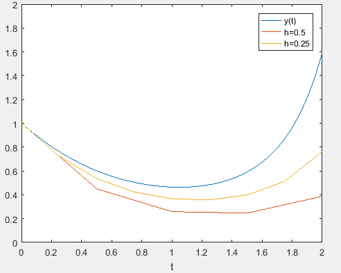
It is inferred that the smaller step-size would give a better approximation to the solution.
(c)
To calculate: The solution of the initial value problem
Answer to Problem 1P
Solution:
The solutions are tabulated as,
| t | y | |
| 0 | 1 | |
| 0.5 | 0.623906 | |
| 1 | 0.491862 | |
| 1.5 | 0.602762 | 0.693176 |
| 2 | 1.364267 | 3.956374 |
Explanation of Solution
Given Information:
The initial value problem
Formula used:
Solve an initial value problem of the form
Here,
Calculation:
From the initial condition
Let
Now,
Proceed further and use the following MATLAB code to implement mid-point iterative scheme and solve the differential equation.
Execute the above code to obtain the solutions tabulated as,
| t | Y | |
| 0 | 1 | |
| 0.5 | 0.623906 | |
| 1 | 0.491862 | |
| 1.5 | 0.602762 | 0.693176 |
| 2 | 1.364267 | 3.956374 |
The results for the are plotted along with the analytical solution
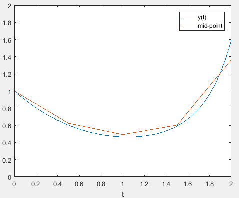
Thus, it is inferred that the mid-point method gives a good approximation to the solution.
(d)
To calculate: The solution of the initial value problem
Answer to Problem 1P
Solution:
The solutions are tabulated as,
| t | y | ||||
| 0 | 1 | ||||
| 0.5 | 0.6016 | ||||
| 1 | 0.4645 | 0.2095 | 0.2391 | 0.6717 | |
| 1.5 | 0.5914 | 0.6801 | 1.4953 | 1.8937 | 4.4609 |
| 2 | 1.5845 | 4.5949 | 10.8302 | 17.0071 | 51.9532 |
Explanation of Solution
Given Information:
The initial value problem
Formula used:
Solve an initial value problem of the form
In the above expression,
Calculation:
From the initial condition
Let
And,
And,
Therefore,
Proceed further and use the following MATLAB code to implement RK method of order four, solve the differential equation.
In an another .m file, define the equation as,
Execute the above code to obtain the solutions tabulated as,
| t | y | ||||
| 0 | 1 | ||||
| 0.5 | 0.6016 | ||||
| 1 | 0.4645 | 0.2095 | 0.2391 | 0.6717 | |
| 1.5 | 0.5914 | 0.6801 | 1.4953 | 1.8937 | 4.4609 |
| 2 | 1.5845 | 4.5949 | 10.8302 | 17.0071 | 51.9532 |
The results for the are plotted along with the analytical solution
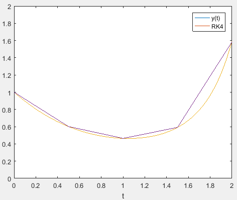
Hence, it is inferred that the RK method of order four gives the best approximation to the solution.
Want to see more full solutions like this?
Chapter 25 Solutions
Numerical Methods For Engineers, 7 Ed


- Which of the 6 graphs below are planar graphs? describe what a planar grapph is and justify your answer for each graph. 1 1 A В 10 10 2 7 5 2 7 9 3. 3. 1 1 C 10 10 2 7 5 2 7. 3. 4 3. E F 10 10 7 8 3. 4arrow_forwardGiven the following network, with the indicated distances between nodes, develop a minimal spanning tree:arrow_forwardx^2-5x^(1/3)+1=0 Has a root between 2 and 2.5 use bisection method to three iterations by hand.arrow_forward
- 3. Using the trial function u¹(x) = a sin(x) and weighting function w¹(x) = b sin(x) find an approximate solution to the following boundary value problems by determining the value of coefficient a. For each one, also find the exact solution using Matlab and plot the exact and approximate solutions. (One point each for: (i) finding a, (ii) finding the exact solution, and (iii) plotting the solution) a. (U₁xx -2 = 0 u(0) = 0 u(1) = 0 b. Modify the trial function and find an approximation for the following boundary value problem. (Hint: you will need to add an extra term to the function to make it satisfy the boundary conditions.) (U₁xx-2 = 0 u(0) = 1 u(1) = 0arrow_forwardQ1: The number of bacterial cells (P) in a given reactor is related to time in days (t) as described by the following mathematical model: dp dt 0.0000007 P², If at initial time (P = 106). Determine the number of cells when (t 2days) using the fourth order Runge-Kutta method and at time increment of (1 day). = = 0.3 P 1arrow_forward5arrow_forward
- For the two-dimensional computational domain of Fig, with the given node distribution, sketch a simple structured grid using four-sided cells and sketch a simple unstructured polyhedral grid using at least one of each: 3-sided, 4-sided, and 5-sided cells. Try to avoid large skewness. Compare the cell count for each case and discuss your results.arrow_forwardMATLAB..Hand written plz asap....i'll upvote surearrow_forward2. Solve the following ODE in space using finite difference method based on central differences with error O(h). Use a five node grid. 4u" - 25u0 (0)=0 (1)=2 Solve analytically and compare the solution values at the nodes.arrow_forward
- A company operates to produce two products x₁ and x2. The production process involves two main resources: labor hours and raw materials. The objective is to maximize the total profit. Below is the formulated linear programming problem: Objective Maximize Subject to Z=2x+3x2 Labour hours Raw materials x1+ 2x2 ≤ 30 x1 + x2 ≤ 20 X1, X2 NO Final Iteration Optimal Tableau Coefficients of: RHS Basic Variables Z x1 X2 X3 X4 Z 1 0 0 1 1 50 X2 0 0 1 1 -1 10 x1 0 1 0 -1 2 10arrow_forwardmathforadmi..2dff1dd723 PTU Kadoorie sygini 1930 Technical Department of Applied Mathematics Second Semester 2020/2021 Math for Administration Assignment 2 Question 1 For the function: y = 0.01x- 0.001x² Find the zeros, the vertex and the optimum value (max. or min.) Question 2 Suppose a company has fixed costs of $300 and variable 3 costs of x + 1460 dollars per unit, 4 where x is the total number of units produced. Suppose further that the selling price of its product is 1500 X- ♡ lar Fine break-even points. init. II جامعة Palestine ||arrow_forwardlook at the graph wich presents F vs x graph ... Q : Determine the compression of the spring from the change in position of the cart+block in Graph ? please tell me the steps how can I find compression of the spring from the change in position of the cart+blockarrow_forward
 Elements Of ElectromagneticsMechanical EngineeringISBN:9780190698614Author:Sadiku, Matthew N. O.Publisher:Oxford University Press
 Mechanics of Materials (10th Edition)Mechanical EngineeringISBN:9780134319650Author:Russell C. HibbelerPublisher:PEARSON
 Thermodynamics: An Engineering ApproachMechanical EngineeringISBN:9781259822674Author:Yunus A. Cengel Dr., Michael A. BolesPublisher:McGraw-Hill Education
 Control Systems EngineeringMechanical EngineeringISBN:9781118170519Author:Norman S. NisePublisher:WILEY
 Mechanics of Materials (MindTap Course List)Mechanical EngineeringISBN:9781337093347Author:Barry J. Goodno, James M. GerePublisher:Cengage Learning
 Engineering Mechanics: StaticsMechanical EngineeringISBN:9781118807330Author:James L. Meriam, L. G. Kraige, J. N. BoltonPublisher:WILEY