
To determine: The aggregate consumer function, income-expenditure equilibrium and the value of the multiplier.
Concept Introduction:
The formula to calculate change in GDP is:
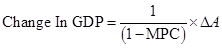
Here,
 is autonomous spending.
 - MPC is marginal propensity to consume.
Marginal Propensity to Consume (MPC): It is defined as the change which occurs in total consumption level due to a change in disposable income.
The formula to calculate MPC is:

Here,
 is change in disposable income.
  is change in consumption level.
 - MPC is marginal propensity to consume.
Multiplier: It is defined as the ratio of total change in the gross domestic product due to a change in the autonomous spending.
The formula to calculate multiplier is:
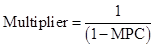
Here,
- MPC is marginal propensity to consume.
Consumption Level (C): It is one of the largest components of GD .The individual consumption depends on the disposable income.
Consumption Function: It shows how the change in disposable income of an individual changes the consumption level.
The formula to calculate consumption function is:
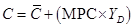
Here,
- C is consumption level.
 is autonomous consumption.
  is disposable income.
 - MPC is marginal propensity to consume.
Autonomous Consumption: This is defined as the consumption level when the income of an individual is zero.
Planned Aggregate Spending: It is the summation of consumption level in an economy and the planned investment.
The formula to calculate planned aggregate spending is:
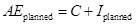
Here,
- C is consumption level.
 is the planned investment spending.
  is the planned aggregate spending.
Unplanned Investment: All those investments that businesses do not intend to take in a given time. It is certain due to some external factors like fall in interest rate and increase in future profitability.
The formula to calculate unplanned investment is:
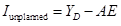
Here,
- YDis disposable income.
 is unplanned investment spending.
 - AE is the planned aggregate spending.
Explanation of Solution
a. Planned aggregate expenditure and unplanned investment.
| GDP | YD(A) | C(B) | Iplanned(C) | AEplanned(D) | Iunplanned |
| (billions of dollars) | |||||
| 0 | 0 | 100 | 300 | 400 |  |
| 400 | 400 | 400 | 300 | 700 |  |
| 800 | 800 | 700 | 300 | 1,000 |  |
| 1,200 | 1,200 | 1,000 | 300 | 1,300 |  |
| 1,600 | 1,600 | 1,300 | 300 | 1,600 | 0 |
| 2,000 | 2,000 | 1,600 | 300 | 1,900 | 100 |
| 2,400 | 2,400 | 1,900 | 300 | 2,200 | 200 |
| 2,800 | 2,800 | 2,200 | 300 | 2,500 | 300 |
| 3,200 | 3,200 | 2,500 | 300 | 2,800 | 400 |
Conclusion:
Hence, the unplanned investment and the planned aggregate expenditure at specific income level have been stated in the table.
b. Aggregate consumption function.
Given,
Autonomous consumption is $100 billion.
Change in disposable income is $400 billion.
Change in aggregate consumer spending is $300 billion.
The formula to calculate MPC is:

Substitute $300 billion for  and $400 billion for
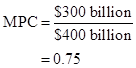
Hence MPC is 0.75.
The formula to calculate consumption function is:
Substitute $100 billion for  and 0.75 for MPC:
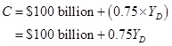
Conclusion:
Thus, the Consumption function is 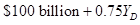
c. Income-expenditure equilibrium GDP.
- Income expenditure equilibrium GDP is the point where planned aggregate spending is equal to the GDP.
- The table in part a highlights that the condition is satisfied at the level where GDP is equal to $1,600 billion.
Conclusion:
Hence, the equilibrium GDP (Y*) is $1,600 billion.
d. Value of the multiplier:
Given,
MPC is 0.75
The formula to calculate multiplier is:
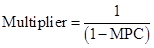
Substitute 0.75 for MPC:
Conclusion;
Thus, multiplier is 4.
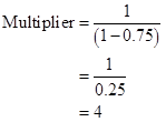
e. The new Y* when planned investment changes.
Given,
New investment is $200 billion
Initial investment is $300 billion
The formula to calculate change in planned investment is:

Substitute $200 billion for new investment and $200 billion for initial investment:
Given,
Change in investment is  billion.
Real GDP is $1,600 billion.
Multiplier is 4.
The formula to calculate new Y* is:

Substitute $1,600 billion for real GDP, 4 for multiplier and  billion for change in investment:
Conclusion:
Thus, new Y* is $1,200 billion.
f. The new Y* when autonomous consumption changes.
Given,
New autonomous consumption is $200 billion.
Initial autonomous consumption is $100 billion.
The formula to calculate change in autonomous consumption is:
Substitute $200 billion for new consumption and $100 billion for initial consumption:
Given,
Change in consumption is $100 billion.
Real GDP is $1,600 billion.
Multiplier is 4.
The formula to calculate new Y* is:

Substitute $1,600 billion for real GDP, 4 for multiplier and $100 billion for change in consumption:
Conclusion:
Thus, new Y* is $2,000 billion.
Want to see more full solutions like this?
Chapter 26 Solutions
Loose-leaf Version for Economics


 Principles of Economics (12th Edition)EconomicsISBN:9780134078779Author:Karl E. Case, Ray C. Fair, Sharon E. OsterPublisher:PEARSON
 Engineering Economy (17th Edition)EconomicsISBN:9780134870069Author:William G. Sullivan, Elin M. Wicks, C. Patrick KoellingPublisher:PEARSON
 Principles of Economics (MindTap Course List)EconomicsISBN:9781305585126Author:N. Gregory MankiwPublisher:Cengage Learning
 Managerial Economics: A Problem Solving ApproachEconomicsISBN:9781337106665Author:Luke M. Froeb, Brian T. McCann, Michael R. Ward, Mike ShorPublisher:Cengage Learning
 Managerial Economics & Business Strategy (Mcgraw-...EconomicsISBN:9781259290619Author:Michael Baye, Jeff PrincePublisher:McGraw-Hill Education