
Concept explainers
Videos
(a)
To construct: The
To find: The
To describe: The direction, form, and strength of the relationship..
(a)
Answer to Problem 26.38E
Scatterplot:
Output using the MINITAB software is given below:
The correlation is 0.649.
The least-squares regression line is
Explanation of Solution
Given info:
The data shows the number of calories the child consumed during lunch.
Calculation:
Scatterplot:
From the given information, Calories is the response variable and Time is the explanatory variable.
Software procedure:
Step-by-step procedure to construct the scatterplot of the Calories against Time using the MINITAB software:
- Choose Stat > Regression > Fitted Line Plot.
- In Responses, enter the column of Calories.
- In Predictors, enter the column of Time.
- In Type of Regression Model, Check as Linear.
- Click OK.
- Observation:
From the scatterplot, it can be observed that the negative linear pattern. Also, there are two outliers present in the scatter plot. Hence, there should be any concerns about these data for using a non-linear model.
- Least-squares regression line:
From the MINITAB output, the least-squares regression line is
- Correlation:
From the plot, the squared correlation
Thus, the correlation value is 0.649.
- (b)
- To check: The conditions for regression inference
- (b)
Answer to Problem 26.38E
- The conditions for regression inference are not satisfied.
Explanation of Solution
- Calculation:
Linear Relationship:
Scatterplot:
From the given information, Residual is the response variable and Time is the explanatory variable.
Software procedure:
Step-by-step procedure to construct the scatterplot of the residuals against Time using the MINITAB software:
- Choose Graph > Scatter plot.
- Choose With Regression, and then click OK.
- Under Y variables, enter a column of Residual.
- Under X variables, enter a column of Time.
- Click OK.
Output using the MINITAB software is given below:
Observation:
The scatterplot of the residuals against time shows that the points are plotted closer to the line. But, there are two outliers present in the scatter plot. Thus, there are no deviations from a straight line apparent.
Hence, there should not be any concern about these data for using a linear model.
Normality Assumption:
Software procedure:
Step-by-step procedure to construct the histogram of the residuals using the MINITAB software:
- Choose Graph > Histogram > Simple.
- Under Graph variables, enter a column of Residual.
- Click OK.
Output using the MINITAB software is given below:
Observation:
From histogram of residual, it can be observed that the bars are plotted more on the left side. Therefore, the plot provided the moderate skewness. Thus, the skewness suggests lack of normality.
Independent Assumption:
Here, the 20 observations are measured separately. Hence, it can be concluded that the observations are independent of each other.
Variability Assumption:
From the scatter plot in Part (a), it can be observed that there are no deviations from a straight line apparent. Hence, there is not any evidence that the variability may be larger at one end.
- (c)
- To check: Whether there is significant evidence that more time at the table is associated with more calories consumed or not.
- To find: The 95% confidence
interval to estimate how rapidly calories consumed changes as time at the table increases.
- (c)
Answer to Problem 26.38E
- The conclusion is that, there is significant evidence that more time at the table is associated with more calories consumed.
- The 95% confidence interval to estimate how rapidly calories consumed changes as time at the table increases is
Explanation of Solution
- Calculation:
The appropriate hypotheses for the given model are as follows:
Null hypothesis:
Alternative hypothesis:
Test statistic and P-value:
From the given information, Calories (Cal) is the response variable and Time is the explanatory variable
Software procedure:
Step-by-step procedure to obtain the test statistic and the P-value using the MINITAB software:
- Choose Stat > Regression > Regression.
- In Responses, enter the column of Cal.
- In Predictors, enter the column of Time.
- Click OK.
Output using the MINITAB software is given below
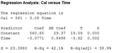
From the MINITAB output, the test statistic value is –3.62 and the P-value is 0.002.
Conclusion:
Use significance level,
Here, P-value is 0.002, which is less than the value of
Therefore, by the rejection rule, it can be concluded that there is an evidence to reject
Confidence interval:
The formula for the 95% confidence interval for the population slope
Where,
Critical value of t:
The degrees of freedom for the test statistic
From Table C, t distribution critical values, the required
Confidence interval:
The 95% confidence interval to estimate how rapidly calories consumed changes as time at the table increases is as follows,
Thus, the 95% confidence interval to estimate how rapidly calories consumed changes as time at the table increases is
Want to see more full solutions like this?
Chapter 26 Solutions
The Basic Practice of Statistics


 MATLAB: An Introduction with ApplicationsStatisticsISBN:9781119256830Author:Amos GilatPublisher:John Wiley & Sons Inc
 Probability and Statistics for Engineering and th...StatisticsISBN:9781305251809Author:Jay L. DevorePublisher:Cengage Learning
 Statistics for The Behavioral Sciences (MindTap C...StatisticsISBN:9781305504912Author:Frederick J Gravetter, Larry B. WallnauPublisher:Cengage Learning
 Elementary Statistics: Picturing the World (7th E...StatisticsISBN:9780134683416Author:Ron Larson, Betsy FarberPublisher:PEARSON
 The Basic Practice of StatisticsStatisticsISBN:9781319042578Author:David S. Moore, William I. Notz, Michael A. FlignerPublisher:W. H. Freeman
 Introduction to the Practice of StatisticsStatisticsISBN:9781319013387Author:David S. Moore, George P. McCabe, Bruce A. CraigPublisher:W. H. Freeman