
a.
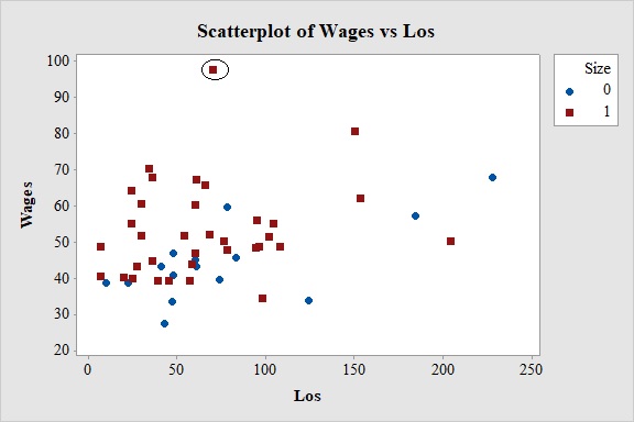
To plot: The values of wages against the values of LOS.
a.
Answer to Problem 29.42E
Output obtained from MINITAB is given below:
Explanation of Solution
Given info:
It is understood that wages will increase if the experience is more. The dataset shows the wages and other factors which is influencing the wages for 50 randomly selected women.
Use different shapes and color to indicate the sizes (large and small). It is seen that one women has high wages with respect to length of service (LOS). Circle this point and don’t use this point while answering the rest of the questions.
Software procedure:
Step by step procedure for constructing scatterplot of wages against LOS is given below:
- Choose Graph >
Scatter plot . - Choose with Groups, and then click OK.
- Under Y variables, enter a column of Wages.
- Under X variables, enter a column of LOS.
- Select Size, under Categorical variable for grouping.
- Click on X-Y pairs form groups.
- Click on Multiple Graph, select Overlaid on the same graph under Show Pairs of Graph Variables.
- Click OK.
Interpretation:
The plot for wages against LOS is constructed where red squares represents large sized bank and blue dot represents small sized bank. The red square on the top is considered to be the highest wages paid.
To remove the wage 204 for the further analysis.
b.
To explain: The reason for using a multiple regression model with two regression lines for predicting wages using LOS and size.
b.
Answer to Problem 29.42E
The variable size is an indicator variable which is given in the data and it should be indicated as 0 or 1. After doing this the multiple regression model can be constructed with two regression lines one for large size bank and other for small size bank.
Explanation of Solution
Justification:
Multiple Linear Regression:
Consider the number of observation on n individuals for which each observation has p explanatory variables
Where,
Indicator variable:
An indicator variable places the individual observation in one among the two categories; an indicator variable is coded by the values 0 and 1.
If
Then, the regression model becomes:
For,
For,
The regression equation used for predicting wages for large size bank is given below:
The regression equation used for predicting wages for small size bank is given below:
Thus, the reason for using a multiple regression model with two regression lines for predicting wages using LOS and size the variable size is an indicator variable which is given in the data and it should be indicated as 0 or 1.
c.
To fit: A regression model that allows testing the slopes for two regression lines.
To test: Whether the slope corresponding to large size bank is equal to the slope corresponding to small size bank.
c.
Answer to Problem 29.42E
Output obtained from MINITAB is given below:
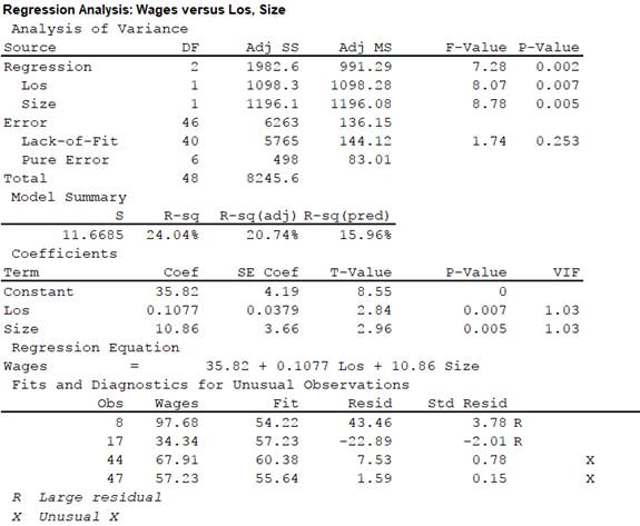
There is enough evidence to infer that the slope corresponding to large size bank is equal to the slope corresponding to small size bank.
Explanation of Solution
Calculation:
Software procedure:
Step by step procedure for fitting a linear model for predicting the wages is given below:
- Choose Stat > Regression >. Regression
- In Response (Y), enter the column containing the variable Wages.
- In Continuous predictor, enter the numeric column containing the variables LOS and Size.
- Click OK.
From the MINITAB output the multiple regression equation is,
The test hypotheses are given below:
Null hypothesis:
Alternative hypothesis:
Test statistic:
The test statistic is,
Substitute the values of
Thus, the test statistic is –5.5914.
Degrees of freedom:
The degrees of freedom is
Thus, the degree of freedom is 45.
Critical value:
Here, level of significance is not given.
So, the prior level of significance
Use the critical values given in the Table C. The critical value for 0.05 level of significance and 45 degree of freedom is calculated.
Degree of freedom is available with an increment of 10 after 30. Thus, 45 degrees of freedom is considered to be 50.
- Under the column of degrees of freedom locate the value 50.
- Look for the value corresponding to 95% confidence interval under the rows of 50 degrees of freedom.
- The critical value for 50 degrees of freedom and 0.05 level of significance is 2.009
Thus, the critical value is 2.009
Decision rule:
If the test statistic is greater than the critical value, then reject the null hypothesis
Conclusion:
Here, the test statistic is -5.5914 and critical value is 2.009.
The t statistic is –5.5914 is less than the critical value. That is
Thus, null hypothesis is not rejected.
Hence, it can be concluded there is sufficient evidence to infer that the two slopes are equal.
d.
To construct: The residual plots for the model constructed in part (c).
To check: Whether the conditions for inference have been met.
d.
Answer to Problem 29.42E
Output obtained from MINITAB is given below:
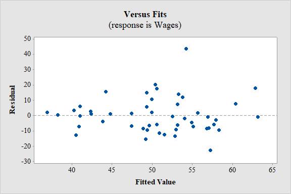
Figure 1
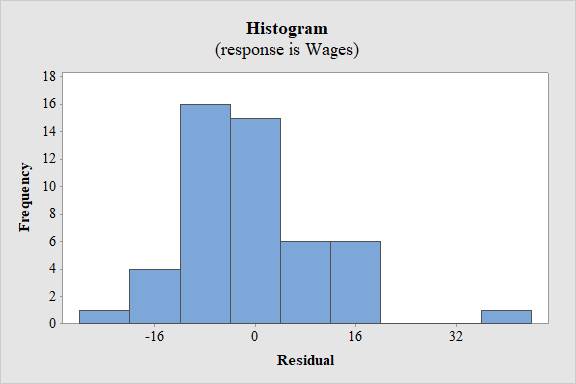
Figure 2
The residual plot and the histogram of residuals both follow the conditions of inference.
Explanation of Solution
Justification:
Step by step procedure for constructing the residual plot and residual plot of histogram is given below:
- Choose Stat > Regression >. Regression
- In Response (Y), enter the column containing the variable Temperature.
- In Continuous predictor, enter the numeric column containing the variables Year and City.
- In graphs select residual versus fit and histogram.
- Click OK.
Residual plots:
A residual plot is a scatterplot of fitted response or explanatory against residuals. Residual plots help in finding whether the regression line fits the data.
Assumptions regarding residuals:
- The residual is centered with mean 0.
- The residual has a constant variance
Conditions for making inferences:
The residual plots are plotted for each residual value against fitted values or the explanatory variables.
The histogram of residuals is drawn to check the normality of error.
Most common type of pattern obtained from residual plot:
- If the plots are scattered randomly in a horizontal band with a 0 mean then the regression line gives a better fit.
- If the plots form a curve pattern, then the relationship between the response and the explanatory variable is non linear.
- If the plot is like a fan shape then it indicates the variation in the response about the regression line increases as the explanatory variable increases.
The scatterplot of residuals versus fitted values of wages is given in Figure 1. The plot tells that the residuals are centered with the mean 0 and the fitted values are scattered in a random manner close to the mean except few values. The residuals are considered to have a constant variability.
The histogram for residuals shown in Figure 2 tells that the residuals are considered to be
Thus, the residual plot and the histogram of residuals both follow the conditions of inference.
Want to see more full solutions like this?
Chapter 29 Solutions
Bundle: Basic Practice of Statistics 7e & LaunchPad (Twelve Month Access)

 MATLAB: An Introduction with ApplicationsStatisticsISBN:9781119256830Author:Amos GilatPublisher:John Wiley & Sons Inc
 Probability and Statistics for Engineering and th...StatisticsISBN:9781305251809Author:Jay L. DevorePublisher:Cengage Learning
 Statistics for The Behavioral Sciences (MindTap C...StatisticsISBN:9781305504912Author:Frederick J Gravetter, Larry B. WallnauPublisher:Cengage Learning
 Elementary Statistics: Picturing the World (7th E...StatisticsISBN:9780134683416Author:Ron Larson, Betsy FarberPublisher:PEARSON
 The Basic Practice of StatisticsStatisticsISBN:9781319042578Author:David S. Moore, William I. Notz, Michael A. FlignerPublisher:W. H. Freeman
 Introduction to the Practice of StatisticsStatisticsISBN:9781319013387Author:David S. Moore, George P. McCabe, Bruce A. CraigPublisher:W. H. Freeman