Chapter 3, Problem 29CE

a.

To determine

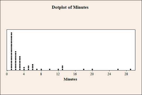
Construct a dot plot for the call length data.

Answer to Problem 29CE

The dot plot for the call length data is given below:

Explanation of Solution

Calculation:

The given information is that, the data represents the length of 65 calls initiated during the last week fo july.

Software procedure:

Step -by-step procedure to draw dot plot using MINITAB software is as follows:

• Select Graph > Dot plot.
• Select Simple under One Y.
• Select the column of Minutes in Graph variables.
• Select OK.

b.

To determine

Construct a frequency distribution.

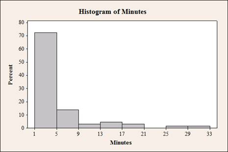
Construct a histogram.

Answer to Problem 29CE

The frequency distribution using nice bin limits

Bin limits		Mid point	Width	Frequency $f$	Percent	Cumulative
Lower	Upper					Frequency	Percent
1	< 5	3	4	47	72.31	47	72.31
5	< 9	7	4	9	13.85	56	85.15
9	< 13	11	4	2	3.08	58	89.23
13	< 17	15	4	3	4.62	61	93.85
17	< 21	19	4	2	3.08	63	96.92
21	< 25	23	4	0	0	63	96.92
25	< 29	27	4	1	1.54	64	98.46
29	< 33	31	4	1	1.54	65	100
Total				65

The histogram is as follows,

Explanation of Solution

Calculation:

Frequency distribution:

It is a tabulation of n data values which are divided into k classes called bins. The bin limits are the cutoff points which defines each bin. These generally have equal interval and the limits do not overlap.

Step-by-step procedure to construct frequency distribution table is as follows:

• The smallest and largest data values are 1 and 29.
• Here the sample size is 65. By Sturge’s Rule, $k=1+3.3\log \left(n\right)$

Thus,

$\begin{array}{c}k=1+3.3\log \left(65\right)\\ =1+5.9826\\ =6.98\\ \approx 7\end{array}$

• Bin width is obtained by dividing the range by the number of bins.

Thus,

$\begin{array}{c}\text{Bin}\text{width}=\frac{x_{\max }-x_{\min }}{k}\\ =\frac{29-1}{7}\\ =4\end{array}$

Hence, the bin width is 4.

• The minimum value in the data is 1 hence the first bin should start at 1.

Thus, the frequency distribution table for call length is as follows:

Bin limits
Lower	Upper
1	< 5
5	< 9
9	< 13
13	< 17
17	< 21
21	< 25
25	< 29
Total

In the 7th bin the largest value is not included. Hence the number of bins should be taken as 8 in order to include the largest value.

Tally mark:

• Make a tally mark for each score in the corresponding class and continue for all reading times in the data.
• The number of tally marks in each class represents the frequency, f of that class.

Thus, the frequency distribution table for calllength is as follows:

Bin limits		Tally	Frequency $f$	Percent
Lower	Upper
1	< 5	$\begin{array}{l}\cancel{\left|\right|\left|\right|}\cancel{\left|\right|\left|\right|}\cancel{\left|\right|\left|\right|}\cancel{\left|\right|\left|\right|}\cancel{\left|\right|\left|\right|}\cancel{\left|\right|\left|\right|}\\ \cancel{\left|\right|\left|\right|}\cancel{\left|\right|\left|\right|}\cancel{\left|\right|\left|\right|}\left|\right|\end{array}$	47	$\frac{47}{65}\times 100=72.31$
5	< 9	$\cancel{\left|\right|\left|\right|}\left|\right|\left|\right|$	9	$\frac{9}{65}\times 100=13.85$
9	< 13	$\left|\right|$	2	$\frac{2}{65}\times 100=3.08$
13	< 17	$\left|\right||$	3	$\frac{3}{65}\times 100=4.62$
17	< 21	$\left|\right|$	2	$\frac{2}{65}\times 100=3.08$
21	< 25		0	$\frac{0}{65}\times 100=0$
25	< 29	$|$	1	$\frac{1}{65}\times 100=1.54$
29	< 33	$|$	1	$\frac{1}{65}\times 100=1.54$
Total			65

Mid point:

The midpoint is the average of the lower limit and upper limit of a particular class. It is also called as class mark.

$\text{Mid}\text{point}=\frac{\left(\text{Lower}\text{class limit+Upper}\text{class}\text{limit}\right)}{2}$

Thus, the mid points for each class is tabulated below:

Bin limits		Frequency $f$	Mid point
Lower	Upper
1	< 5	47	$\frac{1+5}{2}=3$
5	< 9	9	$\frac{5+9}{2}=7$
9	< 13	2	$\frac{9+13}{2}=11$
13	< 17	3	$\frac{13+17}{2}=15$
17	< 21	2	$\frac{17+21}{2}=19$
21	< 25	0	$\frac{21+25}{2}=23$
25	< 29	1	$\frac{25+29}{2}=27$
29	< 33	1	$\frac{29+33}{2}=31$
Total		65

Cumulative frequency:

Cumulative frequency is the running total of frequencies. A cumulative frequency for a particular class would be the total of all frequencies upto that current class The last class’s cumulative frequency is equal to the sample size $n$.

Thus, the cumulative frequency for each calss is tabulated below:

Bin limits		Frequency $f$	Cumulative frequency
Lower	Upper
1	< 5	47	47
5	< 9	9	$47+9=56$
9	< 13	2	$56+2=58$
13	< 17	3	$58+3=61$
17	< 21	2	$61+2=63$
21	< 25	0	$63+0=63$
25	< 29	1	$63+1=64$
29	< 33	1	$64+1=65$
Total		65

Cumulative Relative frequency:

Bin limits		Cumulative frequency	Cumulative percent
Lower	Upper
1	< 5	47	$\frac{47}{65}\times 100=72.31$
5	< 9	56	$\frac{56}{65}\times 100=85.15$
9	< 13	58	$\frac{58}{65}\times 100=89.23$
13	< 17	61	$\frac{61}{65}\times 100=93.85$
17	< 21	63	$\frac{63}{65}\times 100=96.92$
21	< 25	63	$\frac{63}{65}\times 100=96.92$
25	< 29	64	$\frac{64}{65}\times 100=98.46$
29	< 33	65	$\frac{65}{65}\times 100=100$
Total

Software procedure:

Step by step procedure to obtain Histogram using MINITAB is given below:

• Choose Graph > Histogram.
• Choose Simple, and then click OK.
• In Graph variables, enter the corresponding column of Minutes.
• Click Scale > Y-Scale Type > Percent
• Click OK.
• To modify the interval settings, double click on the horizontal axis of the graph. Then, select Binning > Cutpoint > Cutpoint Positions, in this box, enter the values for the cut points of the bin intervals (0, 5, 10, 15, 20, 25, 30, 35, 40, 45 and 50).

c.

To determine

Explain about the distribution based on the displays.

Explanation of Solution

Symmetric:

If the values of the data are elongated equally to the right and left, then the distribution is symmetric.

Skewed right:

If the values of the data are elongated to the right and most of the values are clustered on the left side, then the distribution is skewed right.

Skewed left:

If the values of the data are elongated to the left and most of the values are clustered on the right side, then the distribution is skewed left.

From the histogram in parts (a) and (b) it is observed that, the shape of the distribution is skewed right because the tail is elongated to the right. Most of calllenghts are under 5minutes.