Concept explainers
Videos
a.
Explain the reason behind the unequal class width of the intervals.
a.
Explanation of Solution
The data represents the relative frequency distribution of commute time of working adults.
From the given relative frequency distribution, it can be seen that all the class intervals are not of same width.
- From the relative frequency distribution, it is observed that the researcher wishes to give a detailed analysis of the commute time of working adults at the lower end of the distribution.
- In order to do this, the intervals have to be constructed with at most 5 minutes’ width.
- If this narrower width is considered for all intervals, then the number of intervals will increase.
- To avoid this, the interval width is increased at higher end of the distribution.
Therefore, the intervals are with unequal widths.
b.
Obtain the relative frequencies and densities for the given relative frequency distribution.
b.
Answer to Problem 28E
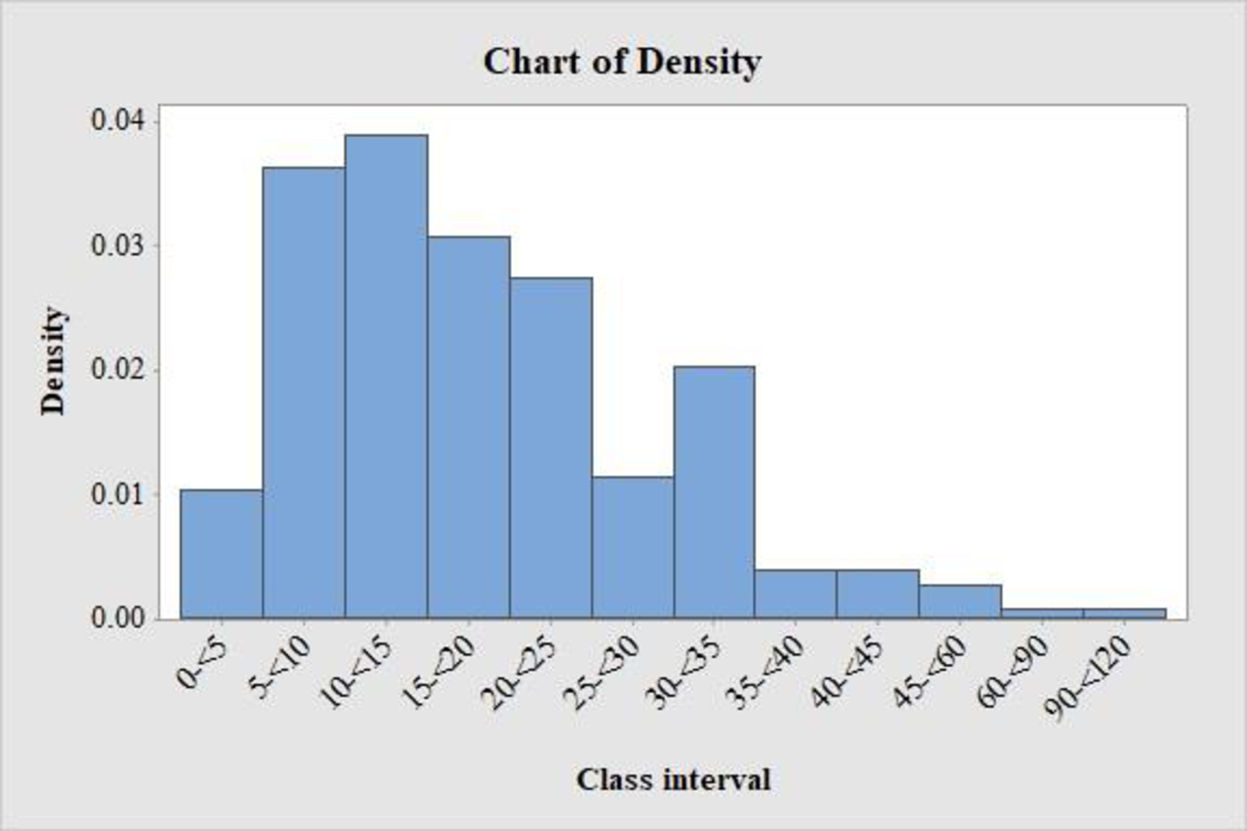
The densities for the class intervals are given below:
| Class interval | Density |
| 0-<5 | 0.0104 |
| 5-<10 | 0.0363 |
| 10-<15 | 0.0390 |
| 15-<20 | 0.0307 |
| 20-<25 | 0.0275 |
| 25-<30 | 0.0114 |
| 30-<35 | 0.0203 |
| 35-<40 | 0.0040 |
| 40-<45 | 0.0040 |
| 45-<60 | 0.0027 |
| 60-<90 | 0.0007 |
| 90-<120 | 0.0007 |
Explanation of Solution
Calculation:
The general formula for the relative frequency is as follows:
Substitute the frequency of the class interval 0-<5 as “5,200” and the total frequency as “100,400” in relative frequency.
Relative frequencies for the remaining class intervals are obtained below:
| Class interval | Frequency | Relative frequency |
| 0-<5 | 5,200 | |
| 5-<10 | 18,200 | |
| 10-<15 | 19,600 | |
| 15-<20 | 15,400 | |
| 20-<25 | 13,800 | |
| 25-<30 | 5,700 | |
| 30-<35 | 10,200 | |
| 35-<40 | 2,000 | |
| 40-<45 | 2,000 | |
| 45-<60 | 4,000 | |
| 60-<90 | 2,100 | |
| 90-<120 | 2,200 | |
| Total | 100,400 |
The general formula for the rectangle height or density is as follows:
Densities of class intervals:
Substitute the relative frequency of the class interval 0-<5 as “0.052”.
Substitute class width as follows:
Density of the class intervals 0-<5 is as follows:
Similarly, densities for the remaining class intervals are obtained below:
| Class interval | Relative frequency | Class width | Density |
| 0-<5 | 0.052 | ||
| 5-<10 | 0.181 | ||
| 10-<15 | 0.195 | ||
| 15-<20 | 0.153 | ||
| 20-<25 | 0.137 | ||
| 25-<30 | 0.057 | ||
| 30-<35 | 0.102 | ||
| 35-<40 | 0.020 | ||
| 40-<45 | 0.020 | ||
| 45-<60 | 0.040 | ||
| 60-<90 | 0.021 | ||
| 90-<120 | 0.022 |
c.
Draw the histogram for the data.
Comment on the important features of the histogram.
c.
Answer to Problem 28E
The histogram is given below:
Explanation of Solution
Calculation:
For the continuous data with unequal class width, the vertical scale of the histogram must be density scale. The rectangle heights are the densities of the intervals.
Here, the class intervals do not have equal length. Hence, the histogram with the relative frequencies is not appropriate.
Therefore, the density of the data has to be used to draw a histogram.
Software procedure:
Step-by-step procedure to draw the histogram using MINITAB software:
- Select Graph > Bar chart.
- In Bars represent select values from a table.
- In one column of values select Simple.
- Enter density in Graph variables.
- Enter Class interval in categorical variable.
- Right click on X-axis; in Edit X Scale in gap between clusters enter 0.
- Select OK.
Observation:
From the histogram, it is observed that the distribution of commute times of working adults is positively skewed with single
The majority of commute times of working adults lies between 5 and 35 minutes.
d.
Find and plot the cumulative frequency distribution for the commute times of working adults.
d.
Answer to Problem 28E
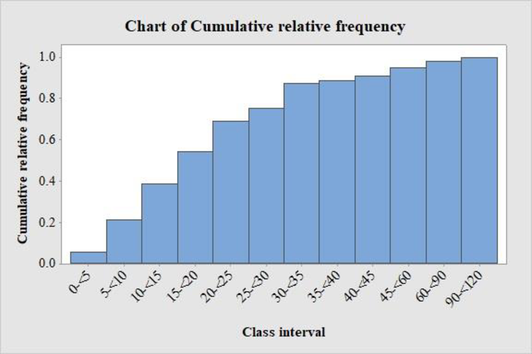
The cumulative relative frequency distribution is as follows:
| Commute time | Cumulative relative frequency |
| 0-<5 | 0.056 |
| 5-<10 | 0.212 |
| 10-<15 | 0.389 |
| 15-<20 | 0.544 |
| 20-<25 | 0.691 |
| 25-<30 | 0.752 |
| 30-<35 | 0.873 |
| 35-<40 | 0.888 |
| 40-<45 | 0.912 |
| 45-<60 | 0.952 |
| 60-<90 | 0.982 |
| 90-<120 | 1 |
The histogram is given below:
Explanation of Solution
Calculation:
Answers may vary; one of the following answers is given below:
Relative frequency distribution:
The general formula for the relative frequency is as follows:
Cumulative relative frequency:
The general formula to obtain cumulative frequency using frequency distribution is as follows:
From the relative frequencies, the cumulative relative frequencies are obtained as follows:
| Commute times | Relative frequency | Cumulative relative frequency |
| 0-<5 | 0.052 | |
| 5-<10 | 0.181 | |
| 10-<15 | 0.195 | |
| 15-<20 | 0.153 | |
| 20-<25 | 0.137 | |
| 25-<30 | 0.057 | |
| 30-<35 | 0.102 | |
| 35-<40 | 0.020 | |
| 40-<45 | 0.020 | |
| 45-<60 | 0.040 | |
| 60-<90 | 0.021 | |
| 90-<120 | 0.022 |
The cumulative relative frequency histogram is plotted for the given data.
Software procedure:
Step-by-step procedure to draw the relative frequency histogram using MINITAB software:
- Select Graph > Bar chart.
- In Bars represent select values from a table.
- In one column of values select Simple.
- Enter Cumulative relative frequency in Graph variables.
- Enter Commute times in categorical variable.
- Right click on X-axis; in Edit X Scale in gap between clusters enter 0.
- Select OK.
e.
(i). Find the approximate proportion of commute times that are less than 50 minutes.
(ii) Find the approximate proportion of commute times that are greater than 22 minutes.
(ii) Find the approximate commute time that separates shortest 50% and longest 50% of commute times.
e.
Answer to Problem 28E
(i) The approximate proportion of commute times that are less than 50 minutes is 0.9253.
(ii) The approximate proportion of commute times that are greater than 22 minutes is 0.3825.
(iii). The commute time that separates shortest 50% and longest 50% of commute times is 30 minutes.
Explanation of Solution
The general formula for the relative frequency or proportion is as follows:
(i). Approximate proportion of commute times that are less than 50 minutes:
The objective is to find the relative frequency of commute times that are less than 50 minutes.
The class width of class interval 45-<60 is 15.
The approximate
The relative frequency of the commute times that are less than 50 minutes is as follows:
Thus, the approximate proportion of commute times are less than 50 minutes is 0.930.
(ii). Approximate proportion of commute times that are greater than 22 minutes:
The objective is to find the relative frequency of commute times that are greater than 22 minutes.
The class width of class interval 20-<25 is 5.
The approximate range of greater than 22 is half of the class interval 20-<25.
Hence, the relative frequency of the commute times that are greater than 22 minutes is as follows:
Thus, the approximate proportion of commute times are greater than 22 minutes is 0.3505.
(iii). Approximate commute time that separates shortest 50% and longest 50% of commute times:
The objective is to find the commute time that separates shortest 50% and longest 50% of commute times.
From the cumulative relative frequency histogram, it is observed that the distribution of commute times of working adults is centered in between 25-<30 and 30-<35 range.
Therefore, the commute time that lies between 25-<30 and 30-<35 range will separate shortest 50% and longest 50% of commute times.
The approximate middle value in between 25-<30 and 30-<35 is 30.
Thus, the approximate commute time that separates shortest 50% and longest 50% of commute times is 30 minutes.
Want to see more full solutions like this?
Chapter 3 Solutions
Introduction To Statistics And Data Analysis (with Jmp Printed Access Card)


 Glencoe Algebra 1, Student Edition, 9780079039897...AlgebraISBN:9780079039897Author:CarterPublisher:McGraw Hill