
Concept explainers
Videos
At you can see in the following table, demand for heart transplant surgery at Washington General Hospital has increased steadily in the past few years:

The director of medical services predicted 6 years ago that demand in year 1 would be 41 surgeries.
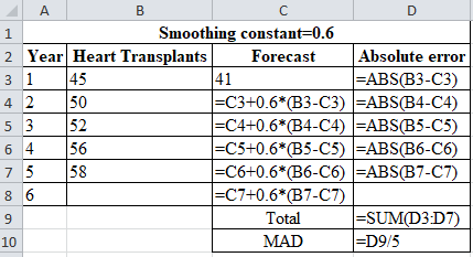
a) Use exponential smoothing, first with a smoothing constant of .6 and then with one of .9, to develop forecasts for years 2 through 6.
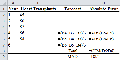
b) Use a 3-year moving average to forecast demand in years 4, 5, and 6.
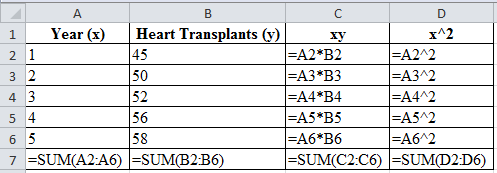
c) Use the trend-projection method to forecast demand in years 1 through 6.
d) With MAD as the criterion, which of the four
a)
To determine: Findthe forecast for years 2 through 6, using exponential smoothing.
Introduction: A sequence of data pointing in successive order is known as time series. Time series forecasting is the prediction based on past events which are at a uniform time interval. Moving average method and trend projections are one of the time series methods which use weights to prioritize past data.
Answer to Problem 13P
The forecast for years 2 through 6 using exponential smoothing with smoothing constant 0.6 is 56.263 and smoothing constant 0.9 is 57.757.
Explanation of Solution
Forecast for years 1 through 6 using exponential smoothing with smoothing constant 0.6:
Given information:
| Year | 1 | 2 | 3 | 4 | 5 | 6 |
| Heart Transplants | 45 | 50 | 52 | 56 | 58 |
Formula to calculate the forecasted demand:
Where,
| Smoothing constant=0.6 | |||
| Year | Heart Transplants | Forecast | Absolute error |
| 1 | 45 | 41 | 4.000 |
| 2 | 50 | 43.400 | 6.600 |
| 3 | 52 | 47.360 | 4.640 |
| 4 | 56 | 50.144 | 5.856 |
| 5 | 58 | 53.658 | 4.342 |
| 6 | 56.263 | ||
| Total | 25.438 | ||
| MAD | 5.08768 | ||
Excel worksheet:
Calculation of the forecast for year 2:
To calculate forecast for year 2, substitute the value of forecast of year 1, smoothing constant and difference of actual and forecasted demand in the above formula. The result of the forecast for year 2 is 43.40.
Calculation of the forecast for year 3:
To calculate forecast for year 3, substitute the value of forecast of year 2, smoothing constant and difference of actual and forecasted demand in the above formula. The result of the forecast for year 3 is 47.360.
Calculation of the forecast for year 4:
To calculate forecast for year 4, substitute the value of forecast of year 3, smoothing constant and difference of actual and forecasted demand in the above formula. The result of the forecast for year 4 is 50.144.
Calculation of the forecast for year 5:
To calculate forecast for year 5, substitute the value of forecast of year 4, smoothing constant and difference of actual and forecasted demand in the above formula. The result of the forecast for year 5 is 53.658.
Calculation of the forecast for year 6:
To calculate forecast for year 6, substitute the value of forecast of year 5, smoothing constant and difference of actual and forecasted demand in the above formula. The result of the forecast for year 6 is 56.263.
Calculation of MAD using exponential smoothing with smoothing constant α=0.6:
Formula to calculate the Mean Absolute Deviation:
Calculation of the absolute error for year 1:
The absolute error for year 1 is the modulus of the difference between 45 and 41, which corresponds to 4. Therefore, the absolute error for year 1 is 4.
Calculation of the absolute error for year 2:
The absolute error for year 2 is the modulus of the difference between 50 and 43.4, which corresponds to 6.6. Therefore, the absolute error for year 2 is 6.6.
Calculation of the absolute error for year 3:
The absolute error for year 3 is the modulus of the difference between 52 and 47.360, which corresponds to 4.640. Therefore, the absolute error for year 3 is4.640.
Calculation of the absolute error for year 4:
The absolute error for year 4 is the modulus of the difference between 56 and 50.144, which corresponds to 5.856. Therefore, the absolute error for year 4 is5.856.
Calculation of the absolute error for year 5:
The absolute error for year 5 is the modulus of the difference between 58 and 53.658, which corresponds to 4.342. Therefore, the absolute error for year 5 is 4.342.
Calculation of the Mean Absolute Deviation using exponential smoothing:
Upon the substitution of summation value of absolute error for 5 years, that is, 25.438 are divided by number of years. That is, 5 yields MAD of 5.08768.
The forecast for years 2 through 6 using exponential smoothing with 0.6 as smoothing constant is 56.263.
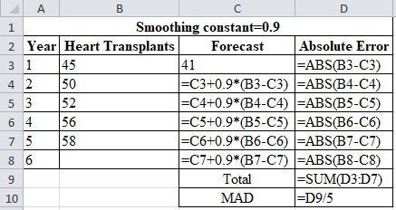
The forecast for years 1 through 6 using exponential smoothing with smoothing constant 0.9:
Given information:
| Year | 1 | 2 | 3 | 4 | 5 | 6 |
| Heart Transplants | 45 | 50 | 52 | 56 | 58 |
Formula to calculate the forecasted demand:
Where
| Smoothing constant=0.9 | |||
| Year | Heart Transplants | Forecast | Absolute Error |
| 1 | 45 | 41 | 4 |
| 2 | 50 | 44.600 | 5.400 |
| 3 | 52 | 49.460 | 2.540 |
| 4 | 56 | 51.746 | 4.254 |
| 5 | 58 | 55.575 | 2.425 |
| 6 | 57.757 | 57.757 | |
| Total | 18.6194 | ||
| MAD | 3.72388 | ||
Excel worksheet:
Calculation of the forecast for year 2:
To calculate the forecast for year 2, substitute the value of forecast of year 1, smoothing constant and difference of actual and forecasted demand in the above formula. The result of the forecast for year 2 is 44.60.
Calculation of the forecast for year 3:
To calculate forecast for year 3, substitute the value of forecast of year 2, smoothing constant and difference of actual and forecasted demand in the above formula. The result of the forecast for year 3 is 49.460.
Calculation of the forecast for year 4:
To calculate forecast for year 4, substitute the value of forecast of year 3, smoothing constant and difference of actual and forecasted demand in the above formula. The result of the forecast for year 4 is 50.144.
Calculation of the forecast for year 5:
To calculate forecast for year 5, substitute the value of forecast of year 4, smoothing constant and difference of actual and forecasted demand in the above formula. The result of the forecast for year 5 is55.575.
Calculation of the forecast for year 6:
To calculate forecast for year 6, substitute the value of forecast of year 5, smoothing constant and difference of actual and forecasted demand in the above formula. The result of the forecast for year 6 is57.757.
Calculation of MAD using exponential smoothing with smoothing constant α=0.9:
Formula to calculate the Mean Absolute Deviation:
Calculation of the absolute error for year 1:
The absolute error for year 1 is the modulus of the difference between 45 and 41, which corresponds to 4. Therefore, the absolute error for year 1 is 4.
Calculation of the absolute error for year 2:
The absolute error for year 2 is the modulus of the difference between 50 and 44.6, which corresponds to 5.4. Therefore, the absolute error for year 2 is 5.4.
Calculation of the absolute error for year 3:
The absolute error for year 3 is the modulus of the difference between 52 and49.460, which corresponds to 2.540. Therefore, the absolute error for year 3 is2.540.
Calculation of the absolute error for year 4:
The absolute error for year 4 is the modulus of the difference between 56 and51.746, which corresponds to 4.254. Therefore, the absolute error for year 4 is4.254.
Calculation of the absolute error for year 5:
The absolute error for year 5 is the modulus of the difference between 58 and55.575, which corresponds to 2.425. Therefore, the absolute error for year 5 is 2.425.
Calculation of the Mean Absolute Deviation using exponential smoothing:
Upon the substitution of summation value of absolute error for 5 years, that is,18.6194are divided by the number of years. That is, 5 yields MAD of 3.72388.
The forecast for years 2 through 6 using exponential smoothing with 0.9 as smoothing constant is 57.757.
Hence, the forecast for years 2 through 6 using exponential smoothing with smoothing constant 0.6 is 56.263 and smoothing constant 0.9 is 57.757.
b)
To determine: Using 3-year moving average, forecast the demand for years 4, 5 and 6.
Answer to Problem 13P
The demand forecast for years 4, 5 and 6 is 49, 52.67 and 55.33.
Explanation of Solution
Given information:
| Year | 1 | 2 | 3 | 4 | 5 | 6 |
| Heart Transplants | 45 | 50 | 52 | 56 | 58 |
Formula to calculate the forecasted demand:
| Year | Heart Transplants | Forecast | Absolute Error |
| 1 | 45 | ||
| 2 | 50 | ||
| 3 | 52 | ||
| 4 | 56 | 49 | 7 |
| 5 | 58 | 52.67 | 5.333 |
| 6 | 55.33 | ||
| Total | 12.333 | ||
| MAD | 6.1667 |
Excel worksheet:
Calculation of the forecast for year 4:
To calculate the forecast for year 4, divide the summation of the values from years 1, 2 and 3 and divide by 3. The corresponding value 49 is the forecast for year 4. The 3-year moving average for year 4 is 49.
Calculation of the forecast for year 5:
To calculate the forecast for year 5, divide the summation of the values from years 2, 3 and 4 and divide by 3. The corresponding value 52.67 is the forecast for year 5. The 3-year moving average for year 5 is 52.67.
Calculation of the forecast for year 6:
To calculate the forecast for year 6, divide the summation of the values from years 3, 4, 5 and divide by 3. The corresponding value 55.33 is the forecast for year 5. The 3-year moving average for year 5 is 55.33.
Calculation of MAD using 3-year moving average:
Formula to calculate the Mean Absolute Deviation:
Calculation of the absolute error for year 4:
The absolute error for year 4 is the modulus of the difference between 56 and 49, which corresponds to 7. Therefore, the absolute error for year 4 is 7.
Calculation of the absolute error for year 5:
The absolute error for year 4 is the modulus of the difference between 58 and 52.67, which corresponds to 5.33. Therefore, the absolute error for year 4 is 5.33.
Calculation of the Mean Absolute Deviation using 3-year moving average:
Upon the substitution of the summation value of the absolute error for 2 years, that is,12.333is divided by number of years. That is, 2 yields MAD of 6.1666.
Hence, the demand forecast for years 4, 5 and 6 is 49, 52.67 and 55.33.
c)
To determine: Find the demand forecast in year 1 through 6using trend projection.
Answer to Problem 13P
The forecast in year 1 through 6using trend projection is62.1.
Explanation of Solution
Given information:
| Year | 1 | 2 | 3 | 4 | 5 | 6 |
| Heart Transplants | 45 | 50 | 52 | 56 | 58 |
Formula to calculate the demand forecast
Where,
Where,
| Year (x) | Heart Transplants (y) | xy | x^2 |
| 1 | 45 | 45 | 1 |
| 2 | 50 | 100 | 4 |
| 3 | 52 | 156 | 9 |
| 4 | 56 | 224 | 16 |
| 5 | 58 | 290 | 25 |
| ∑=15 | ∑=261 | ∑=815 | ∑=55 |
Excel worksheet
Substituting the values in the above formula
Calculation of average of x values
The average of x values is obtained by dividing the summation of x values, that is, (1+2+…+5) with the number of period n. That is, 5. The value of
Calculation of average of y values
The average of y values is obtained by dividing the summation of sales with the number of period n. That is, 5. The value of
Calculation of slope of regression line‘b’:
The summation of product of sales (y) with x values is ∑xy = 815, the product of number of years (n), the average of x values and the average of y values is obtained. That is,
The summation of square of x values, that is, 55 is subtracted from the product of the number of years. That is,5 with average of x values;3. The resultant value is 10. The slope of regression line is obtained by dividing 32 with 10. The value of ‘b’ is 3.2.
Calculation of y-axis intercept ‘a’:
The y-axis intercept is obtained by the difference between average of y values and values obtained by the product of slope of regression line with average of x values. The resultant value of ‘a’ is 42.9.
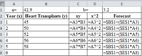
Calculation of the forecast for years 1 through 6:
| a= | 42.9 | b= | 3.2 | |
| Year (x) | Heart Transplants (y) | xy | x^2 | Forecast |
| 1 | 45 | 45 | 1 | 46.1 |
| 2 | 50 | 100 | 4 | 49.3 |
| 3 | 52 | 156 | 9 | 52.5 |
| 4 | 56 | 224 | 16 | 55.7 |
| 5 | 58 | 290 | 25 | 58.9 |
| 6 | 62.1 | |||
Excel worksheet:
Calculation of forecast of year 1:
The forecast for year 1 is obtained by the summation of the product of slope of regression line and forecasted year, with the y-axis intercept. The forecasted value obtained is 46.1.
Calculation of forecast of year 2:
The forecast for year 2 is obtained by the summation of the product of slope of regression line and forecasted year, with the y-axis intercept. The forecasted value obtained is 49.3.
Calculation of forecast of year 3:
The forecast for year 3 is obtained by the summation of the product of slope of regression line and forecasted year, with the y-axis intercept. The forecasted value obtained is 52.5.
Calculation of forecast of year 4:
The forecast for year 4 is obtained by the summation of the product of slope of regression line and forecasted year, with the y-axis intercept. The forecasted value obtained is 55.7.
Calculation of forecast of year 5:
The forecast for year 5 is obtained by the summation of the product of slope of regression line and forecasted year, with the y-axis intercept. The forecasted value obtained is 58.9.
Calculation of forecast of year 6:
The forecast for year 6 is obtained by the summation of the product of slope of regression line and forecasted year, with the y-axis intercept. The forecasted value obtained is 62.1.
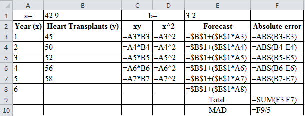
Formula to calculate the Mean Absolute Deviation:
Calculation of MAD using trend projection:
| a= | 42.9 | b= | 3.2 | ||
| Year (x) | Heart Transplants (y) | xy | x^2 | Forecast | Absolute error |
| 1 | 45 | 45 | 1 | 46.1 | 1.1 |
| 2 | 50 | 100 | 4 | 49.3 | 0.7 |
| 3 | 52 | 156 | 9 | 52.5 | 0.5 |
| 4 | 56 | 224 | 16 | 55.7 | 0.3 |
| 5 | 58 | 290 | 25 | 58.9 | 0.9 |
| 6 | 62.1 | ||||
| Total | 3.5 | ||||
| MAD | 0.7 | ||||
Excel worksheet:
Calculation of the absolute error for year 1:
The absolute error for year 1 is the modulus of the difference between 45 and 46.1, which corresponds to 1.1. Therefore, the absolute error for year 1 is 1.1.
Calculation of the absolute error for year 2:
The absolute error for year 2 is the modulus of the difference between 50 and 49.3, which corresponds to 0.7. Therefore, the absolute error for year 2 is 0.7.
Calculation of the absolute error for year 3:
The absolute error for year 3 is the modulus of the difference between 52 and 52.5, which corresponds to 0.5. Therefore, the absolute error for year 3 is 0.5.
Calculation of the absolute error for year 4:
The absolute error for year 4 is the modulus of the difference between 56 and 55.7, which corresponds to 0.3. Therefore, the absolute error for year 4 is 0.3.
Calculation of the absolute error for year 5:
The absolute error for year 5 is the modulus of the difference between 58 and 58.9, which corresponds to 0.9. Therefore, the absolute error for year 5 is 0.9.
Calculation of the Mean Absolute Deviation using trend projection:
Upon the substitution of summation value of absolute error for 5 years, that is,3.5is divided by the number of years. That is,5 yields MAD of 0.7.
Thus, the forecast in year 1 through 6 using trend projection is 62.1.
d)
To determine: Compare the MAD of exponential smoothing, 3-year moving average and trend projection and infer the best method.
Explanation of Solution
On Comparing MAD from the four methods, (refer to equations (1), (2), (3) and (4)) it can be inferred that trend projection is the best methods since it has the least MAD.
Want to see more full solutions like this?
Chapter 4 Solutions
Principles Of Operations Management


- Under what conditions might a firm use multiple forecasting methods?arrow_forwardThe Baker Company wants to develop a budget to predict how overhead costs vary with activity levels. Management is trying to decide whether direct labor hours (DLH) or units produced is the better measure of activity for the firm. Monthly data for the preceding 24 months appear in the file P13_40.xlsx. Use regression analysis to determine which measure, DLH or Units (or both), should be used for the budget. How would the regression equation be used to obtain the budget for the firms overhead costs?arrow_forwardScenario 3 Ben Gibson, the purchasing manager at Coastal Products, was reviewing purchasing expenditures for packaging materials with Jeff Joyner. Ben was particularly disturbed about the amount spent on corrugated boxes purchased from Southeastern Corrugated. Ben said, I dont like the salesman from that company. He comes around here acting like he owns the place. He loves to tell us about his fancy car, house, and vacations. It seems to me he must be making too much money off of us! Jeff responded that he heard Southeastern Corrugated was going to ask for a price increase to cover the rising costs of raw material paper stock. Jeff further stated that Southeastern would probably ask for more than what was justified simply from rising paper stock costs. After the meeting, Ben decided he had heard enough. After all, he prided himself on being a results-oriented manager. There was no way he was going to allow that salesman to keep taking advantage of Coastal Products. Ben called Jeff and told him it was time to rebid the corrugated contract before Southeastern came in with a price increase request. Who did Jeff know that might be interested in the business? Jeff replied he had several companies in mind to include in the bidding process. These companies would surely come in at a lower price, partly because they used lower-grade boxes that would probably work well enough in Coastal Products process. Jeff also explained that these suppliers were not serious contenders for the business. Their purpose was to create competition with the bids. Ben told Jeff to make sure that Southeastern was well aware that these new suppliers were bidding on the contract. He also said to make sure the suppliers knew that price was going to be the determining factor in this quote, because he considered corrugated boxes to be a standard industry item. Is Ben Gibson acting legally? Is he acting ethically? Why or why not?arrow_forward
- Scenario 3 Ben Gibson, the purchasing manager at Coastal Products, was reviewing purchasing expenditures for packaging materials with Jeff Joyner. Ben was particularly disturbed about the amount spent on corrugated boxes purchased from Southeastern Corrugated. Ben said, I dont like the salesman from that company. He comes around here acting like he owns the place. He loves to tell us about his fancy car, house, and vacations. It seems to me he must be making too much money off of us! Jeff responded that he heard Southeastern Corrugated was going to ask for a price increase to cover the rising costs of raw material paper stock. Jeff further stated that Southeastern would probably ask for more than what was justified simply from rising paper stock costs. After the meeting, Ben decided he had heard enough. After all, he prided himself on being a results-oriented manager. There was no way he was going to allow that salesman to keep taking advantage of Coastal Products. Ben called Jeff and told him it was time to rebid the corrugated contract before Southeastern came in with a price increase request. Who did Jeff know that might be interested in the business? Jeff replied he had several companies in mind to include in the bidding process. These companies would surely come in at a lower price, partly because they used lower-grade boxes that would probably work well enough in Coastal Products process. Jeff also explained that these suppliers were not serious contenders for the business. Their purpose was to create competition with the bids. Ben told Jeff to make sure that Southeastern was well aware that these new suppliers were bidding on the contract. He also said to make sure the suppliers knew that price was going to be the determining factor in this quote, because he considered corrugated boxes to be a standard industry item. As the Marketing Manager for Southeastern Corrugated, what would you do upon receiving the request for quotation from Coastal Products?arrow_forwardThe file P13_42.xlsx contains monthly data on consumer revolving credit (in millions of dollars) through credit unions. a. Use these data to forecast consumer revolving credit through credit unions for the next 12 months. Do it in two ways. First, fit an exponential trend to the series. Second, use Holts method with optimized smoothing constants. b. Which of these two methods appears to provide the best forecasts? Answer by comparing their MAPE values.arrow_forwardThe owner of a restaurant in Bloomington, Indiana, has recorded sales data for the past 19 years. He has also recorded data on potentially relevant variables. The data are listed in the file P13_17.xlsx. a. Estimate a simple regression equation involving annual sales (the dependent variable) and the size of the population residing within 10 miles of the restaurant (the explanatory variable). Interpret R-square for this regression. b. Add another explanatory variableannual advertising expendituresto the regression equation in part a. Estimate and interpret this expanded equation. How does the R-square value for this multiple regression equation compare to that of the simple regression equation estimated in part a? Explain any difference between the two R-square values. How can you use the adjusted R-squares for a comparison of the two equations? c. Add one more explanatory variable to the multiple regression equation estimated in part b. In particular, estimate and interpret the coefficients of a multiple regression equation that includes the previous years advertising expenditure. How does the inclusion of this third explanatory variable affect the R-square, compared to the corresponding values for the equation of part b? Explain any changes in this value. What does the adjusted R-square for the new equation tell you?arrow_forward
- The file P13_22.xlsx contains total monthly U.S. retail sales data. While holding out the final six months of observations for validation purposes, use the method of moving averages with a carefully chosen span to forecast U.S. retail sales in the next year. Comment on the performance of your model. What makes this time series more challenging to forecast?arrow_forwardWeekly income for Quiet Mental Breakdown, an online psychology firm, is provided below. Determine, on the basis of minimizing the mean square error, whether a three-period or four-period simple moving average gives a better forecast. Week Income 1 980 2 1040 3 1120 4 1050 5 960 6 990 7 1030 8 1260 9 1240 10 1100 Group of answer choices Both the four-period & three-period simple moving averages have the same forecast accuracy in terms of their MSE There is not enough information to determine the answer The four-period simple moving averages gives a better forecast because it has the smallest MSE The three-period simple moving average gives a better forecast because it has the smallest MSEarrow_forwardBased on the following equation for a moving average forecast, what would have been the three week moving average forecast for week 53 for Small Town Restaurant (see downloaded file for actual demand)? Provide two decimal places and use normal rounding. What happens if we increase the time periods in our moving average forecast to six weeks opposed to three? Group of answer choices It would be more accurate because it includes more data. There would be no change. It would be less sensitive to changes. It would be better at predicting a trend.arrow_forward
 Practical Management ScienceOperations ManagementISBN:9781337406659Author:WINSTON, Wayne L.Publisher:Cengage,
 Purchasing and Supply Chain ManagementOperations ManagementISBN:9781285869681Author:Robert M. Monczka, Robert B. Handfield, Larry C. Giunipero, James L. PattersonPublisher:Cengage Learning
 Contemporary MarketingMarketingISBN:9780357033777Author:Louis E. Boone, David L. KurtzPublisher:Cengage Learning
 MarketingMarketingISBN:9780357033791Author:Pride, William MPublisher:South Western Educational Publishing