
Subpart (a):
The consumer surplus , total surplus and deadweight loss .
Subpart (a):
Explanation of Solution
Figure -1 illustrates the
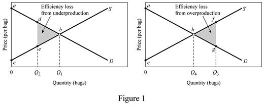
In figure -1 panel (a) and (b), the horizontal axis measures the quantity of bags and the vertical axis measures the
The inverse demand function can be derived as follows:
The inverse demand functions of
The inverse supply curve can be calculated as follows:
The inverse supply functions of
The inverse demand function and supply functions reveal that the producer willing price is $5 and the consumer willing price is $85. The equilibrium price is $45. The total surplus can be calculated as follows:
The total surplus is $800.
The consumer surplus can be calculated as follows:
The consumer surplus is $400.
Concept Introduction:
Consumer surplus: It refers to the variation in the probable charge of a product that the consumer intends to pay and the actual price that he has already paid.
Subpart (b):
The consumer surplus, total surplus and deadweight loss.
Subpart (b):
Explanation of Solution
The consumer willing price at Q2 level of output (15 units) can be calculated by substituting the Q2 level of output to the inverse demand function.
The consumer new willing price is $55.
The producer willing price at Q2 level of output (15 units) can be calculated by substituting the Q2 level of output into the inverse supply function.
The producer’s new willing price is $35.
The deadweight loss can be calculated as follows:
The deadweight loss is $50.
The total surplus can be calculated as follows:
The total surplus is $750.
Concept Introduction:
Consumer surplus: It refers to the variation in the probable charge of a product that the consumer intends to pay and the actual price that he has already paid.
Producer surplus: It refers to the variation in the probable price that the producer intends to sell and the actual price that he has already sold.
Subpart c):
The consumer surplus, total surplus and deadweight loss.
Subpart c):
Explanation of Solution
The consumer willing price at Q3 level of output (27 units) can be calculated by substituting the Q3 level of output to the inverse demand function.
The consumer new willing price is $31.
The producer willing price at Q3 level of output (127 units) can be calculated by substituting the Q3 level of output to the inverse supply function.
The producer new willing price is $59.
The deadweight loss can be calculated as follows:
The deadweight loss is $98.
The total surplus can be calculated as follows:
The total surplus is $702.
Concept Introduction:
Consumer surplus: It refers to the variation in the probable charge of a product that the consumer intends to pay and the actual price that he has already paid.
Producer surplus: It refers to the variation in the probable price that the producer intends to sell and the actual price that he has already sold.
Want to see more full solutions like this?
Chapter 4 Solutions
Connect 1-Semester Access Card for Macroeconomics

- Consider a two-good exchange economy with two types of consumers. Type A have the utility function And an endowment of 3 units of good 1 and k units of good 2. Type B has the utility function And an endowment of 6 units of good 1 and 21 - k units of good 2. a. Find the competitive equilibrium outcome and show that the equilibrium price p* = p1/p2 of good 1 in terms of good 2 is p* = 21+k/15. b. Find the income levels (MA; MB) of both types in equilibrium as a function of k. c. Suppose that the government can make a lump-sum transfer of good 2, but it is impossible to transfer good 1. Use your answer to part b to describe the set of income distributions attainable through such transfers. Draw this in a diagram. d. Suppose that the government can affect the initial distribution of resources by varying k. Find the optimal distribution of income if (i) the SWF is W = log(MA) + log(MB) and (ii) W = MA + MB.arrow_forwardConsider a two-good two-consumer exchange economy where u1 = X1Y1 and u2 = X2Y2, endowment of person 1 = (3, 4) and endowment of person 2= (2, 2). Setting the price of good Y to one (Py = 1), what is the price of good X in the competitive equilibrium? 01 0 6/5 O 3/5 O 3/2arrow_forwardUsing general equilibrium analysis, and taking into account feedback effects, analyze the effects of increased taxes on airline tickets on travel to major tourist destinations such as Florida and California and on the hotel rooms in those destinations.arrow_forward
- In each of the following questions assume that the market is in equilibrium at X. Identify the new equilibrium following the changes given below: The market is for private education, and it receives a subsidy from the state because it is perceived to be a merit good. The market is for new housing, and building costs fall following a general fall in oil prices. The market is for cigarettes, and the government increases indirect taxes and at the same time smoking become less fashionable for people over 30. The market is for motor insurance, and the price of cars falls and at the same time the government subsidises private motor insurance. The market is for electronic goods which often employs very low paid assembly workers. The minimum wage rises and interest rates rise which affects consumer confidence. The market is for student textbooks following a fall in the costs of printing and a considerable increase in the numbers of students going to university. The market is for…arrow_forwardIf the equilibrium quantity in a competitive market is 25, but society (by some means) buys and sells a total of 41 units, then an inefficiency is caused by the exchange of 16 units.True or Falsearrow_forwardSuppose that there is an isolated market economy with just one good: money. The market has 1,000 partici- pants and the total value of money is $1 billion. Consider the following allocations. (a) Every participant has $1 million. (b) One person has $2 million, and everyone else has $500,000 (c) One person has $1 billion, everyone else has $0. Which of the above allocations are Pareto optimal and which are not? Why?arrow_forward
- Refer to Figure 9-2. Without trade, consumer surplus amounts to Group of answer choices $9,720. $19,440. $23,280. $20,280.arrow_forwardThere are six potential consumers of computer games, each willing to buy only one game. Consumer 1 is willing to pay $40 for a computer game, consumer 2 is willing to pay $35, consumer 3 is willing to pay $30, consumer 4 is willing to pay $25, consumer 5 is willing to pay $20, and consumer 6 is willing to pay $15. Suppose the market price is $29. What is the total consumer surplus? The market price decreases to $19. What is the total consumer surplus now? When the price falls from $29 to $19, how much does each consumer’s individual consumer surplus change? How does total consumer surplus change?arrow_forwardInclude correctly labeled diagrams, if useful or required, in explaining your answers. A correctly labeled diagram must have all axes and curves clearly labeled and must show directional changes. If the question prompts you to “Calculate,” you must show how you arrived at your final answer. Assume that sugar-based soft drinks are produced in a market shown on the graph above. Answer the following questions based on the information given in the graph. (a) To reduce the consumption of sugary soft drinks, suppose the government imposes a $2 per-unit sales tax on soft drinks. (i) Will the price of soft drinks increase by the full amount of the sales tax? Explain. (ii) Calculate the tax revenue the government can collect from the sale of soft drinks. Show your work. (iii) Will the consumer surplus increase, decrease, or stay the same after the tax? (iv) Calculate the deadweight loss created by the tax. Show your work. (b) Suppose that instead of imposing the per-unit sales tax,…arrow_forward
- Look at Tables , which show, respectively, the willingness to pay and willingness to accept of buyers and sellers of bags of oranges. For the following questions, assume that the equilibrium price and quantity will depend on the indicated changes in supply and demand. Assume that the only market participants are those listed by name in the two tables. a. What are the equilibrium price and quantity for the data displayed in the two tables?b. What if, instead of bags of oranges, the data in the two tables dealt with a public good like fireworks displays? If al the buyers free ride, what will be the quantity supplied by private sellers?c. Assume that we are back to talking about bags of oranges (a private good), but that the government has decided that tossed orange peels impose a negative externality onthe public that must be rectified by imposing a $2-perbag tax on sellers. What is the new equilibrium price and quantity? If the new equilibrium quantity is the optimal quantity, by how…arrow_forwardRefer to Table 8-1 in Question 9. Suppose the cost to build the park is $24 per acre and that the residents have agreed to split the cost of building the park equally, as in Question 10. If the residents decide to build a park with size equal to the number of acres that maximizes total social surplus from the park, how much total surplus (i.e., net benefit) will Xavier receive? (enter just the number, no $)arrow_forwardConsider the market for apartments. The market price of each apartment is $375,000, and each buyer demands no more than one apartment. Suppose that Rajiv is the only consumer in the apartment market. His willingness to pay for an apartment is $600,000. Based on Rajiv's willingness to pay, the following graph shows his demand curve for apartments. Shade the area representing Rajiv's consumer surplus using the green rectangle (triangle symbols). Part 2 Now, suppose another buyer, Simone, enters the market for apartments, and her willingness to pay is $450,000. Based on Simone's and Rajiv's respective willingness to pay, plot the market demand curve on the following graph using the blue points (circle symbol). Next, shade Rajiv's consumer surplus using the green rectangle (triangle symbols), and shade Simone's consumer surplus using the purple rectangle (diamond symbols). Note: Plot your points as a step function in the order in which you would like them connected. Line…arrow_forward
 Managerial Economics: A Problem Solving ApproachEconomicsISBN:9781337106665Author:Luke M. Froeb, Brian T. McCann, Michael R. Ward, Mike ShorPublisher:Cengage Learning