
Concept explainers
Videos
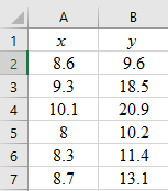
Incoine: Medicai Care Let x be per capita income in thousands of dollars. Let y be the number of medical doctors per 10,000 residents. Six small cities in Oregon gave the following information about x and y(based on information from Lifein America's Small Cities by G. S. Thomas, Prometheus Books).
| x | 8.6 | 9.3 | 10.1 | 8.0 | 8.3 | 8.7 |
| y | 9.6 | 18.5 | 20.9 | 10.2 | 11.4 | 13.1 |
Complete parts (a) through (e), given
(a)
To graph: The scatter diagram.
Explanation of Solution
Given: The data that consists of the variables ‘per capita income in thousands of dollars’ and ‘the number of medical doctors per 10,000 residents’, which are represented by x and y, respectively, are provided.
Graph:
Follow the steps given below in MS Excel to obtain the scatter diagram of the data.
Step 1: Enter the data into an MS Excel sheet. The screenshot is given below.
Step 2: Select the data and click on ‘Insert’. Go to ‘charts’ and select ‘Scatter’ as the chart type.
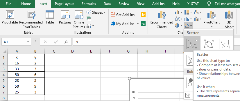
Step 3: Select the first plot and click the ‘add chart element’ option provided in the left-hand corner of the menu bar. Insert the ‘Axis titles’ and the ‘Chart title’. The scatter plot for the provided data is shown below.
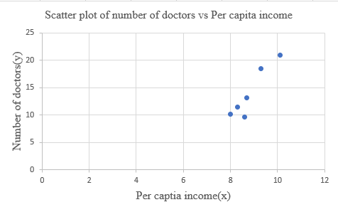
Interpretation: The scatterplot shows that the correlation between the per capita income (x) and the number of medical doctors (y) is positive. So, as x increases (or decreases), the value of y increases (or decreases).
(b)
To test: Whether the provided values of
Answer to Problem 13P
Solution: The provided values, that is,
Explanation of Solution
Given: The provided values are
Calculation:
To compute
| 8.6 | 9.6 | 73.96 | 92.16 | 82.56 |
| 9.3 | 18.5 | 86.49 | 342.25 | 172.05 |
| 10.1 | 20.9 | 102.01 | 436.81 | 211.09 |
| 8 | 10.2 | 64 | 104.04 | 81.6 |
| 8.3 | 11.4 | 68.89 | 129.96 | 94.62 |
| 8.7 | 13.1 | 75.69 | 171.61 | 113.97 |
Now, the value of
Substitute the values in the above formula. Thus:
Thus, the value of
Conclusion: The provided values, that is,
(c)
To find: The values of
Answer to Problem 13P
Solution: The calculated values are
Explanation of Solution
Given: The provided values are
Calculation:
The value of
The value of
The value of
The value of
Therefore, the values are
The general formula of a least-squares line is:
Here, a is the y-intercept and b is the slope.
Substitute the values of a and b in the general equation to get the equation of the least-squares line of the data as follows:
Therefore, the least-squares line equation is
(d)
To graph: The least-squares line on the scatter diagram that passes through the point
Explanation of Solution
Given: The data that consists of the variables ‘per capita income’ and ‘the number of medical doctors per 10,000 residents’, which are represented by x and y, respectively, are provided.
Graph:
Follow the steps given below in MS Excel to obtain the scatter diagram of the data.
Step 1: Enter the data into an MS Excel sheet. The screenshot is given below.
Step 2: Select the data and click on ‘Insert’. Go to ‘charts’ and select ‘Scatter’ as the chart type.
Step 3: Select the first plot and click the ‘add chart element’ option provided in the left-hand corner of the menu bar. Insert the ‘Axis titles’ and the ‘Chart title’. The scatter plot for the provided data is shown below.
Step 4: Right click on any data point and select ‘Add Trendline’. In the dialogue box, select ‘linear’ and check ‘Display Equation on Chart’. The scatter diagram with the least-squares line is given below.
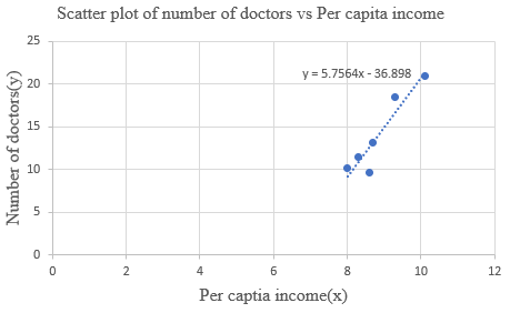
Interpretation: The least-squares line passes through the point
(e)
The value of
Answer to Problem 13P
Solution: The value of
Explanation of Solution
Given: The value of the correlation coefficient (r) is
Calculation: The coefficient of determination
Therefore, the value of
Further, the proportion of variation in y that cannot be explained can be calculated as:
Hence, the percentage of variation in y that cannot be explained is 12.8%.
Interpretation: About 87.2% of the variation in y can be explained by the corresponding variation in x and the least-squares line while the remaining 12.8% of variation cannot be explained.
(f)
To find: The predicted number of MDs (medical doctors) per 10,000 residents.
Answer to Problem 13P
Solution: The predicted value is 20.7 physicians per 10,000 residents.
Explanation of Solution
Given: The least-squares line from part (c) is
Calculation:
The predicted value
Thus, the value of
Interpretation: The predicted number of medical doctors per 10,000 residents for a city with a per capita income of 10 thousand dollars is 20.7.
Want to see more full solutions like this?
Chapter 4 Solutions
EBK UNDERSTANDING BASIC STATISTICS


 Big Ideas Math A Bridge To Success Algebra 1: Stu...AlgebraISBN:9781680331141Author:HOUGHTON MIFFLIN HARCOURTPublisher:Houghton Mifflin Harcourt
 Algebra: Structure And Method, Book 1AlgebraISBN:9780395977224Author:Richard G. Brown, Mary P. Dolciani, Robert H. Sorgenfrey, William L. ColePublisher:McDougal Littell
 Glencoe Algebra 1, Student Edition, 9780079039897...AlgebraISBN:9780079039897Author:CarterPublisher:McGraw Hill
 Algebra & Trigonometry with Analytic GeometryAlgebraISBN:9781133382119Author:SwokowskiPublisher:Cengage
 Elementary Geometry For College Students, 7eGeometryISBN:9781337614085Author:Alexander, Daniel C.; Koeberlein, Geralyn M.Publisher:Cengage,