Concept explainers
Videos
(a)
>The least squares regression line for the given data set.
(a)
>Answer to Problem 23E
Explanation of Solution
Given information:
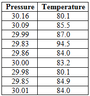
Below table represents the temperature, in degrees Fahrenheit, and barometric pressure, in inches of mercury, on August
noon in Macon, Georgia, over a nine-year period:
Concepts Used:
The equation for least-square regression line:
Where
The correlation coefficient of a data is given by:
Where,
The standard deviations are given by:
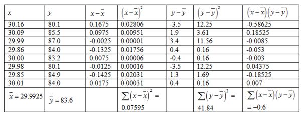
Calculation:
The mean of
The mean of
The data can be represented in tabular form as:
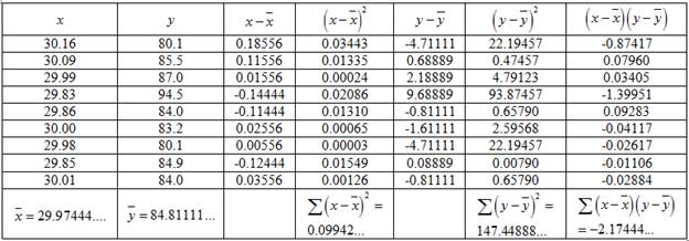
Hence, the standard deviation is given by:
And,
Consider,
Putting the values in the formula,
Putting the values to obtain
Putting the values to obtain
Hence, the least-square regression line is given by:
Therefore, the least squares regression line for the given data set is
(b)
>The coefficient of determination.
(b)
>Answer to Problem 23E
Explanation of Solution
Given information:
Same as part
Calculation:
From part
The coefficient of determination is given by:
Where
Plugging the values to obtain Coefficient of Determination,
Therefore, the Coefficient of Determination is
(c)
>A
(c)
>Answer to Problem 23E

Explanation of Solution
Given information:
Same as part
Calculation:

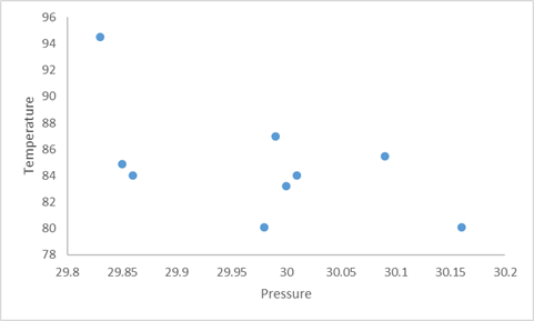
Consider pressure as
The points representing the data would be given by:
Plotting the points to make a scatter plot:
(d)
>The outliers point.
(d)
>Answer to Problem 23E
Explanation of Solution
Given information:
Same as part
Calculation:

Consider pressure as
From above table, it can be observed that among all the
Therefore, the outlier point is
(e)
>The least squares regression line for the given data set by excluding the outlier.
(e)
>Answer to Problem 23E
Explanation of Solution
Given information:
Same as part
Concepts used:
The equation for least-square regression line:
Where
The
Where,
The standard deviations are given by:
Calculation:
From part
Excluding the outlier,
The mean of
The mean of
The data can be represented in tabular form as:
Hence, the standard deviation is given by:
And,
Consider,
Putting the values in the formula,
Putting the values to obtain
Plugging the values to obtain
Hence, the least-square regression line is given by:
Therefore, the least squares regression line for the given data set by excluding the outlier is
(f)
>Whether outlier is influential.
(f)
>Answer to Problem 23E
The outlier is influential.
Explanation of Solution
Given information:
Same as part
Calculation:
From part
From part
From above equations, it can be observed that removing the outlier creates a great difference in the equation of the least square regression line.
Therefore, the outlier is influential.
(g)
>The coefficient of determination for the data set with the outlier removed.
(g)
>Answer to Problem 23E
The proportion of variation is less without the outlier.
Explanation of Solution
Given information:
Same as part
Calculation:
From part
The coefficient of determination is given by:
Where
Plugging the values to obtain Coefficient of Determination,
Therefore, the Coefficient of Determination is
Here the coefficient of determination has reduced without the outlier.
Hence, the proportion of variance explained is less without the outlier.
Want to see more full solutions like this?
Chapter 4 Solutions
Elementary Statistics 2nd Edition


 Linear Algebra: A Modern IntroductionAlgebraISBN:9781285463247Author:David PoolePublisher:Cengage Learning
 Glencoe Algebra 1, Student Edition, 9780079039897...AlgebraISBN:9780079039897Author:CarterPublisher:McGraw Hill