Videos
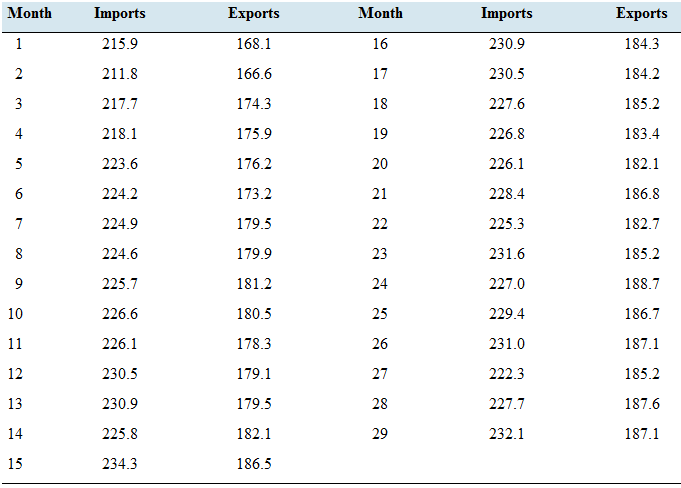
Imports and exports: The following table presents the U.S. imports and exports (in billions of dollars) for each of 29 months.
- Compute the least-squares regression line for predicting exports (y) from imports (x).
- Compute the coefficient of determination.
- The months two lowest exports are months 1 and 2. when the exports were 168.1 and 166.6, respectively. Remove these points and compute the least-squares regression line. Is die result noticeably different?
- Compute the coefficient of determination for the data set months 1 and 2 removed.
- Two economists decide to study the relationship between imports and exports. One uses data from months 1 through 29 and the other uses data from months 3 through 29. For which data set will the proportion of variance explained by the least-squares regression line be greater?
a.
To find: The least-square regression line for the given data set.
Answer to Problem 26E
The least square regression line of the given data set is,
Explanation of Solution
Given:
The import and exports of United States within
Calculation:
The least-square regression is given by the formula,
Where
The correlation coefficient is given by the formula,
Considering the exports as
The correlation coefficient can be obtained by the following table.
| x | y | Zx | Zy | ZxZy |
| 215.9 | 168.1 | -1.99175 | -2.32277 | 4.626396 |
| 211.8 | 166.6 | -2.79101 | -2.58707 | 7.220549 |
| 217.7 | 174.3 | -1.64086 | -1.23035 | 2.018834 |
| 218.1 | 175.9 | -1.56288 | -0.94844 | 1.482294 |
| 223.6 | 176.2 | -0.49071 | -0.89558 | 0.439465 |
| 224.2 | 173.2 | -0.37374 | -1.42417 | 0.532271 |
| 224.9 | 179.5 | -0.23728 | -0.31412 | 0.074536 |
| 224.6 | 179.9 | -0.29576 | -0.24365 | 0.072062 |
| 225.7 | 181.2 | -0.08133 | -0.01459 | 0.001187 |
| 226.6 | 180.5 | 0.094118 | -0.13793 | -0.01298 |
| 226.1 | 178.3 | -0.00335 | -0.52556 | 0.001762 |
| 230.5 | 179.1 | 0.854389 | -0.3846 | -0.3286 |
| 230.9 | 179.5 | 0.932365 | -0.31412 | -0.29288 |
| 225.8 | 182.1 | -0.06184 | 0.143989 | -0.0089 |
| 234.3 | 186.5 | 1.595165 | 0.919257 | 1.466367 |
| 230.9 | 184.3 | 0.932365 | 0.531623 | 0.495667 |
| 230.5 | 184.2 | 0.854389 | 0.514003 | 0.439158 |
| 227.6 | 185.2 | 0.289059 | 0.6902 | 0.199509 |
| 226.8 | 183.4 | 0.133106 | 0.373045 | 0.049655 |
| 226.1 | 182.1 | -0.00335 | 0.143989 | -0.00048 |
| 228.4 | 186.8 | 0.445012 | 0.972116 | 0.432603 |
| 225.3 | 182.7 | -0.15931 | 0.249707 | -0.03978 |
| 231.6 | 185.2 | 1.068824 | 0.6902 | 0.737703 |
| 227 | 188.7 | 0.172094 | 1.306891 | 0.224908 |
| 229.4 | 186.7 | 0.639953 | 0.954496 | 0.610833 |
| 231 | 187.1 | 0.951859 | 1.024975 | 0.975632 |
| 222.3 | 185.2 | -0.74413 | 0.6902 | -0.5136 |
| 227.7 | 187.6 | 0.308553 | 1.113074 | 0.343442 |
| 232.1 | 187.1 | 1.166295 | 1.024975 | 1.195423 |
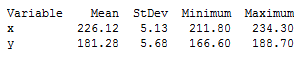
The sum of
Hence, the correlation coefficient is,
Then, the coefficient
Therefore,
Conclusion:
The least square regression line is found to be,
b.
To calculate: The coefficient of determination.
Answer to Problem 26E
The coefficient of determination is found to be,
Explanation of Solution
Calculation:
The correlation coefficient
The coefficient of determination is calculated by taking the square of the correlation coefficient.
Therefore, the coefficient of determination should be,
Simplifying the square,
Conclusion:
Therefore, the coefficient of determination is found to be
c.
To find:The least-square regression line without considering the lowest two exports.
Answer to Problem 26E
The least square regression line of the given data set is,
Explanation of Solution
Calculation:
From the all
The statistics should be calculated again for the current data set, imports and exports of last
The calculations can be completed using a table.
| x | y | Zx | Zy | ZxZy |
| 217.7 | 174.3 | -2.36254 | -1.85805 | 4.389725 |
| 218.1 | 175.9 | -2.26121 | -1.48713 | 3.362707 |
| 223.6 | 176.2 | -0.86789 | -1.41758 | 1.230299 |
| 224.2 | 173.2 | -0.71589 | -2.11306 | 1.512718 |
| 224.9 | 179.5 | -0.53856 | -0.65255 | 0.351434 |
| 224.6 | 179.9 | -0.61456 | -0.55982 | 0.344039 |
| 225.7 | 181.2 | -0.33589 | -0.25844 | 0.086808 |
| 226.6 | 180.5 | -0.10789 | -0.42072 | 0.045393 |
| 226.1 | 178.3 | -0.23456 | -0.93074 | 0.218314 |
| 230.5 | 179.1 | 0.880098 | -0.74528 | -0.65592 |
| 230.9 | 179.5 | 0.98143 | -0.65255 | -0.64043 |
| 225.8 | 182.1 | -0.31056 | -0.0498 | 0.015465 |
| 234.3 | 186.5 | 1.842756 | 0.970245 | 1.787925 |
| 230.9 | 184.3 | 0.98143 | 0.460224 | 0.451678 |
| 230.5 | 184.2 | 0.880098 | 0.437042 | 0.384639 |
| 227.6 | 185.2 | 0.145437 | 0.668869 | 0.097279 |
| 226.8 | 183.4 | -0.05723 | 0.251579 | -0.0144 |
| 226.1 | 182.1 | -0.23456 | -0.0498 | 0.01168 |
| 228.4 | 186.8 | 0.348102 | 1.039794 | 0.361955 |
| 225.3 | 182.7 | -0.43722 | 0.0893 | -0.03904 |
| 231.6 | 185.2 | 1.158762 | 0.668869 | 0.77506 |
| 227 | 188.7 | -0.00656 | 1.480266 | -0.00971 |
| 229.4 | 186.7 | 0.601433 | 1.016611 | 0.611424 |
| 231 | 187.1 | 1.006763 | 1.109342 | 1.116845 |
| 222.3 | 185.2 | -1.19722 | 0.668869 | -0.80078 |
| 227.7 | 187.6 | 0.170771 | 1.225256 | 0.209238 |
| 232.1 | 187.1 | 1.285427 | 1.109342 | 1.425979 |
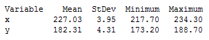
The sum the values in the right most column is found to be,
Hence, the correlation coefficient is,
Then, the coefficient
Therefore,
Conclusion:
The least square regression line is found to be,
d.
To calculate: The coefficient of determination for the last
Answer to Problem 26E
The coefficient of determination is found to be,
Explanation of Solution
Calculation:
The correlation coefficient
The coefficient of determination is calculated by taking the square of the correlation coefficient.
Simplifying the square,
Conclusion:
Therefore, the coefficient of determination is found to be
e.
To find: The data set which
Answer to Problem 26E
The data set with all
Explanation of Solution
Calculation:
The coefficient of determination for the all
Then, the coefficient of determination for the
The coefficient of determination denotes the proportion of variance that is explained by the least-square regression line.
For the all
Conclusion:
Since
Want to see more full solutions like this?
Chapter 4 Solutions
Loose Leaf Version For Elementary Statistics


 Elementary Linear Algebra (MindTap Course List)AlgebraISBN:9781305658004Author:Ron LarsonPublisher:Cengage Learning
 Linear Algebra: A Modern IntroductionAlgebraISBN:9781285463247Author:David PoolePublisher:Cengage Learning
 Glencoe Algebra 1, Student Edition, 9780079039897...AlgebraISBN:9780079039897Author:CarterPublisher:McGraw Hill