Loose Leaf Version For Elementary Statistics
3rd Edition
ISBN: 9781260373523
Author: William Navidi Prof., Barry Monk Professor
Publisher: McGraw-Hill Education
bartleby

Concept explainers

bartleby

Videos

Textbook Question
Book Icon
Chapter 4, Problem 12RE

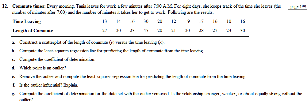
Commute times: Every morning, Tania leaves for work a few minutes after 7:00 A.M. For eight days, she keeps track of the time she leaves (the number of minutes after 7:00) and the number of minutes it takes her to get to work. Following are the results.

Chapter 4, Problem 12RE, Commute times: Every morning, Tania leaves for work a few minutes after 7:00 A.M. For eight days,

  1. Construct a scatterplot of the length of commute (y) versus the time leaving (x).
  2. Compute the least-squares regression line for predicting the length of commute from the time leaving.
  3. Compute the coefficient of determination.
  4. Which point is an outlier?
  5. Remove the outlier and compute the least-squares regression line for predicting the length of commute from the time leaving.
  6. Is the outlier influential? Explain.
  7. Compute the coefficient of determination for the data set with the outlier removed. Is the relationship stronger. weaker; or about equally strong without the outlier?

a.

Expert Solution
Check Mark
To determine

To Graph:a scatter plot using the length of commute time y versus time leaving x

Explanation of Solution

Given information: T leaves her home every day few minutes after 7.00 A.M. The time she leaves the home (The number of minutes after 7.00 A.M) and the number of minutes taken to office has been recorded as below.

    x131416302012917161016
    y2720234520212028272330

Graph:The scatter plot shows the number of minutes after 7.00 A.M on the x -axis and the number of minutes taken to office on the y -axis.

  Loose Leaf Version For Elementary Statistics, Chapter 4, Problem 12RE , additional homework tip  1

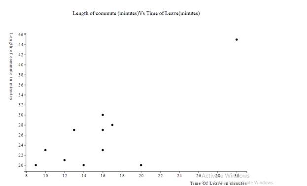
Interpretation:Each of the data in the table contributes an ordered pair of the form (number of minutes after 7.00 A.M, number of minutes taken to office).So the ordered pairs to be plotted are

  (13,27),(14,20),(16,23),(30,45),(20,20),(12,21),(9,20),(17,28),(16,27),(10,23),(16,30) .

We use a scatter plot for this example because to understand the relationship between the two variables as ordered pairs it is useful. The points tend to cluster around the straight line. Therefore, we conclude that the variable on the x -axis and variable on the y -axis have a linear relationship.

Now consider the three points (9,20),(14,20),(20,20) . These show that the number of minutes after 7.00 A.M on the x -axis does not change with the number of minutes taken to an office on the y -axis. There are few other points in the table to reflect the same idea.

Therefore, we conclude that the variable on the x -axis and variable on the y -axis have a linear relationship, but it is difficult to say whether it is negative or positive.

Because for positive linear relationship the large value of data associates with large values of data in the plot, while for negative linear relationship the large value of data associates with small values of data in the pot. And in this case, it is difficult to say that because the large values of data associate with both small and large and small values of data associate with both small and large at the same time.

Therefore it is good to measure how strong the linear relationship is, to know this we can calculate the correlation coefficient.

b.

Expert Solution
Check Mark
To determine

To Calculate: the least square regression line

Answer to Problem 12RE

When two variables have a linear relationship, the points on a scatter plot tend to cluster around a straight line called the least square regression line. It is simplified to be y=26+4×1031x .

Explanation of Solution

Given information: T leaves her home every day few minutes after 7.00 A.M. The time she leaves the home (The number of minutes after 7.00 A.M) and the number of minutes taken to office has been recorded as below.

    x131416302012917161016
    y2720234520212028272330

Formulas Used:

Sample mean: x¯=i=1nxin

Sample variance: s2=i=1n ( x i x ¯ )2n1

Correlation Coefficient: r=1(n1).i=1n(xix¯)sx.i=1n(yiy¯)sy

The least-square regression line:

  y=b0+b1xb1=rsysxb0=y¯b1x¯

Calculation: Using the below table for calculation.

  xyx¯y¯ (x x ¯ )2 (y y ¯ )2xx¯yy¯132715.7272727325.818187.4380171.3966942.7272727271.1818181821420  2.98347133.851241.7272727275.818181821623  0.074387.9421490.2727272732.818181823045  203.7107367.942114.2727272719.181818182020  18.256233.851244.2727272735.818181821221  13.8925623.214883.7272727274.81818182920  45.256233.851246.7272727275.818181821728  1.6198354.7603311.2727272732.1818181821627  0.074381.3966940.2727272731.1818181821023  32.801657.9421495.7272727272.818181821630  0.0743817.48760.2727272734.181818182

The sample means and the sample variances can be calculated as shown.

  x¯= i=1 n x i nx¯=13+14+16+30+20+12+9+17+16+10+1611x¯=17311x¯=15.72727

  s2= i=1 n ( x i x ¯ ) 2 n1sx2= (1315.72727)2+..............+ (1615.72727)210sx2=326.181810sx2=32.61818sx=5.71123279161

  y¯= i=1 n y i ny¯=27+20+23+45+20+21+20+28+27+23+3011y¯=28411y¯=25.81818

  s2= i=1 n ( y i y ¯ ) 2 n1sy2= (2725.81818)2+..............+ (3025.81818)210sy2=533.636410sy2=53.36364sy=7.30504209433

Now, one can use these to calculate the correlation coefficient as shown.

  r=1(n1). i=1 n ( x i x ¯ )sx. i=1 n ( y i y ¯ )syr=1(111).7.1054274× 10 157.30504209433.1.77636× 10 145.71123279161r=110(0.972674395×10¹⁵)(0.311029171×10¹⁴)r=0.030253011×1029r=3.0253011×1031

Finally, to calculate the least square regression line as shown, theser can be used.

  y=b0+b1x

Where b0 (intercept) and b1 (slope) can be calculated as shown.

  b1=rsysx=(3.0253011×1031)7.305042094335.71123279161=3.869559×1031=4.0×1031b0=y¯b1x¯=25.81818(3.869559×1031)(15.72727273)=25.818180=26

c.

Expert Solution
Check Mark
To determine

To Calculate: the coefficient of determination

Answer to Problem 12RE

The coefficient of determination is r2=

  9.1524467×1062

Explanation of Solution

Given information: T leaves her home every day few minutes after 7.00 A.M. The time she leaves the home (The number of minutes after 7.00 A.M) and the number of minutes taken to office has been recorded as below.

    x131416302012917161016
    y2720234520212028272330

Formulas Used:

Sample mean: x¯=i=1nxin

Sample variance: s2=i=1n ( x i x ¯ )2n1

Correlation Coefficient: r=1(n1).i=1n(xix¯)sx.i=1n(yiy¯)sy

Calculation: the correlation coefficient can be calculated as shown by using the formula.

  r=1(n1). i=1 n ( x i x ¯ )sx. i=1 n ( y i y ¯ )syr=1(111).7.1054274× 10 157.30504209433.1.77636× 10 145.71123279161r=110(0.972674395×10¹⁵)(0.311029171×10¹⁴)r=0.030253011×1029r=3.0253011×1031

The correlation coefficient r measures the strength of a linear relationship. Positive values of r

indicates a positive linear association. Here the value of the correlation coefficient close to zero.

Therefore, one can conclude that the positive linear relationship is weak.

Also,

To calculate the coefficient of determination we need to square the correlation coefficient.

Therefore, the coefficient of determination is r2=

  9.1524467×1062

d.

Expert Solution
Check Mark
To determine

To Find: the outlier point

Explanation of Solution

Given information: Tania leaves her home every day few minutes after 7.00 A.M. The time she leaves the home (The number of minutes after 7.00 A.M) and the number of minutes taken to office has been recorded as below.

    x131416302012917161016
    y2720234520212028272330

Graph: The scatter plot shows the number of minutes after 7.00 A.M on the x -axis and the number of minutes taken to an office on the y -axis.

  Loose Leaf Version For Elementary Statistics, Chapter 4, Problem 12RE , additional homework tip  2

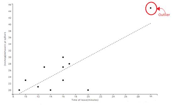
Interpretation: An outlier is a value that considerably larger or considerably smaller than most of the values in a data set. It may be resulting from an error in the process of sampling.

So in the given data set, an outlier point can be detected in the ordered pair (30,45) .

Because it is much larger than the other ordered pairs.

e.

Expert Solution
Check Mark
To determine

To Calculate: the least square regression line without the outlier point.

Answer to Problem 12RE

The least square regression line without theoutlier point is y=24+1030x

Explanation of Solution

Given information: T leaves her home every day few minutes after 7.00 A.M. The time she leaves the home (The number of minutes after 7.00 A.M) and the number of minutes taken to office has been recorded as below.

    x131416302012917161016
    y2720234520212028272330

Formulas Used:

Sample mean: x¯=i=1nxin

Sample variance: s2=i=1n ( x i x ¯ )2n1

Correlation Coefficient: r=1(n1).i=1n(xix¯)sx.i=1n(yiy¯)sy

The least square regression line:

  y=b0+b1xb1=rsysxb0=y¯b1x¯

Calculation: the sample means and the sample variances can be calculated as shown without the outlier point.

  x¯= i=1 n x i nx¯=13+14+1+20+12+9+17+16+10+1610x¯=14310x¯=14.3

  y¯= i=1 n y i ny¯=27+20+23+20+21+20+28+27+23+3010y¯=23910y¯=23.9

  s2= i=1 n ( x i x ¯ ) 2 n1sx2= (1314.3)2+..............+ (1614.3)29sx2=102.19sx2=11.3444444sx=3.36815148115

  s2= i=1 n ( y i y ¯ ) 2 n1sy2= (2723.9)2+..............+ (3023.9)29sy2=128.99sy2=14.3222222sy=3.78447

Now, one can use these to calculate the correlation coefficient without the outlier as shown.

  r=1(n1). i=1 n ( x i x ¯ )sx. i=1 n ( y i y ¯ )syr=1(101).7.1054× 10 153.36815148115.1.42109× 10 143.78447119159r=19(2.1096×10¹⁵)(3.75504×10¹⁵)r=8.80179146×1031

Finally, one can use these to calculate the least square regression line as shown.

  y=b0+b1x

Where b0 (intercept) and b1 (slope) can be calculated as shown.

  b1=rsysx=(8.80179146×1031)3.784471193.36815148115=9.889735182×1031b0=y¯b1x¯=23.9(9.889735182×1031)(14.3)=23.9141.4232131×1031=23.90=23.9

f.

Expert Solution
Check Mark
To determine

To Show: the outlier is influential

Answer to Problem 12RE

No, the outlier is not that much influential.

Explanation of Solution

Given information: T leaves her home every day few minutes after 7.00 A.M. The time she leaves the home (The number of minutes after 7.00 A.M) and the number of minutes taken to office has been recorded as below.

    x131416302012917161016
    y2720234520212028272330

The least-square regression line with the outlier is y=26+4×1031x .

The least-square regression line without the outlier is y=24+1030x .

The two least square regression lines are so much close and have no huge difference.

Therefore we can conclude that the outlier is not that much influential. Here, the outlier cannot be a result of an error. It is just random data measured along with the other data in the sampling process.

g.

Expert Solution
Check Mark
To determine

To Find: the coefficient of determination without the outlier and discuss its strength.

Answer to Problem 12RE

Coefficient of determination is r2=

  77.4715329053

  ×1062.

Explanation of Solution

Given information: T leaves her home every day few minutes after 7.00 A.M. The time she leaves the home (The number of minutes after 7.00 A.M) and the number of minutes taken to office has been recorded as below.

    x131416302012917161016
    y2720234520212028272330

Formula Used:Sample mean: x¯=i=1nxin

Sample variance: s2=i=1n ( x i x ¯ )2n1

Correlation Coefficient: r=1(n1).i=1n(xix¯)sx.i=1n(yiy¯)sy

Calculation: to calculate the correlation coefficient without the outlier as shown.

  r=1(n1). i=1 n ( x i x ¯ )sx. i=1 n ( y i y ¯ )syr=1(101).7.1054× 10 153.36815148115.1.42109× 10 143.78447119159r=19(2.1096×10¹⁵)(3.75504×10¹⁵)r=8.80179146×1031

The correlation coefficient r measures the strength of a linear relationship. Positive values of r

indicates a positive linear association. It is r=8.8×1031 without the outlier.

The value is so close to zero .because of the ten to the power is minus thirty-one.

Therefore, one can conclude that the positive linear relationship is very weak without the outlier.

Also,

One can calculate the coefficient of determination by squaring the correlation coefficient.

Therefore, the coefficient of determination is r2=77.4715329053×1062.

Want to see more full solutions like this?

Subscribe now to access step-by-step solutions to millions of textbook problems written by subject matter experts!

Chapter 4 Solutions

Loose Leaf Version For Elementary Statistics

Ch. 4.1 - In Exercises 17-20, compute the correlation...Ch. 4.1 - In Exercises 17-20, compute the correlation...Ch. 4.1 - In Exercises 21-24, determine whether the...Ch. 4.1 - In Exercises 21-24, determine whether the...Ch. 4.1 - In Exercises 21-24, determine whether the...Ch. 4.1 - In Exercises 21-24, determine whether the...Ch. 4.1 - In Exercises 25-30, determine whether the...Ch. 4.1 - In Exercises 25-30, determine whether the...Ch. 4.1 - In Exercises 25-30, determine whether the...Ch. 4.1 - In Exercises 25-30, determine whether the...Ch. 4.1 - In Exercises 25-30, determine whether the...Ch. 4.1 - In Exercises 25-30, determine whether the...Ch. 4.1 - Price of eggs and milk: The following table...Ch. 4.1 - Government funding: The following table presents...Ch. 4.1 - Pass the ball: The following table lists the...Ch. 4.1 - Carbon footprint: Carbon dioxide (CO2) is produced...Ch. 4.1 - Foot temperatures: Foot ulcers are a common...Ch. 4.1 - Mortgage payments: The following table presents...Ch. 4.1 - Blood pressure: A blood pressure measurement...Ch. 4.1 - Prob. 38ECh. 4.1 - Police and crime: In a survey of cities in the...Ch. 4.1 - Age and education: A survey of U.S. adults showed...Ch. 4.1 - Whats the correlation? In a sample of adults, the...Ch. 4.1 - Prob. 42ECh. 4.1 - Changing means and standard deviations: A small...Ch. 4.2 - In Exercises 5-7, fill in each blank with the...Ch. 4.2 - In Exercises 5-7, fill in each blank with the...Ch. 4.2 - In Exercises 5-7, fill in each blank with the...Ch. 4.2 - Prob. 8ECh. 4.2 - Prob. 9ECh. 4.2 - Prob. 10ECh. 4.2 - Prob. 11ECh. 4.2 - Prob. 12ECh. 4.2 - In Exercises 13-16, compute the least-squares...Ch. 4.2 - In Exercises 13-16, compute the least-squares...Ch. 4.2 - In Exercises 13-16, compute the least-squares...Ch. 4.2 - In Exercises 13-16, compute the least-squares...Ch. 4.2 - Compute the least-squares regression he for...Ch. 4.2 - Compute the least-squares regression he for...Ch. 4.2 - In a hypothetical study of the relationship...Ch. 4.2 - Assume in a study of educational level in years...Ch. 4.2 - Price of eggs and milk: The following table...Ch. 4.2 - Government funding: The following table presents...Ch. 4.2 - Pass the ball: The following table lists the...Ch. 4.2 - Carbon footprint: Carbon dioxide (CO2) is produced...Ch. 4.2 - Foot temperatures: Foot ulcers are a common...Ch. 4.2 - Mortgage payments: The following table presents...Ch. 4.2 - Blood pressure: A blood pressure measurement...Ch. 4.2 - Butterfly wings: Do larger butterflies live...Ch. 4.2 - Interpreting technology: The following display...Ch. 4.2 - Interpreting technology: The following display...Ch. 4.2 - Interpreting technology: The following MINITAB...Ch. 4.2 - Interpreting technology: The following MINITAB...Ch. 4.2 - Prob. 33ECh. 4.2 - Prob. 34ECh. 4.2 - Least-squares regression line for z-scores: The...Ch. 4.3 - In Exercises 5-10, fill in each blank with the...Ch. 4.3 - In Exercises 5-10, fill in each blank with the...Ch. 4.3 - In Exercises 5-10, fill in each blank with the...Ch. 4.3 - In Exercises 5-10, fill in each blank with the...Ch. 4.3 - In Exercises 5-10, fill in each blank with the...Ch. 4.3 - Prob. 10ECh. 4.3 - Prob. 11ECh. 4.3 - In Exercises 11-14, determine whether the...Ch. 4.3 - Prob. 13ECh. 4.3 - In Exercises 11-14, determine whether the...Ch. 4.3 - For the following data set: Compute the...Ch. 4.3 - For the following data set: Compute the...Ch. 4.3 - For the following data set: Compute the...Ch. 4.3 - For the following data set: Compute the...Ch. 4.3 - Prob. 19ECh. 4.3 - Prob. 20ECh. 4.3 - Prob. 21ECh. 4.3 - Prob. 22ECh. 4.3 - Hot enough for you? The following table presents...Ch. 4.3 - Presidents and first ladies: The presents the ages...Ch. 4.3 - Mutant genes: In a study to determine whether the...Ch. 4.3 - Imports and exports: The following table presents...Ch. 4.3 - Energy consumption: The following table presents...Ch. 4.3 - Cost of health care: The following table presents...Ch. 4.3 - Prob. 29ECh. 4.3 - Prob. 30ECh. 4.3 - Prob. 31ECh. 4.3 - Transforming a variable: The following table...Ch. 4.3 - Prob. 33ECh. 4.3 - Prob. 34ECh. 4 - Compute the correlation coefficient for the...Ch. 4 - The number of theaters showing the movie Monsters...Ch. 4 - Use the data in Exercise 2 to compute the...Ch. 4 - A scatterplot has a correlation of r=1. Describe...Ch. 4 - Prob. 5CQCh. 4 - Prob. 6CQCh. 4 - Use the least-squares regression line computed in...Ch. 4 - Use the least-squares regression line computed in...Ch. 4 - Prob. 9CQCh. 4 - A scatterplot has a least-squares regression line...Ch. 4 - Prob. 11CQCh. 4 - Prob. 12CQCh. 4 - A sample of students was studied to determine the...Ch. 4 - In a scatter-plot; the point (-2, 7) is...Ch. 4 - The correlation coefficient for a data set is...Ch. 4 - Prob. 1RECh. 4 - Prob. 2RECh. 4 - Hows your mileage? Weight (in tons) and fuel...Ch. 4 - Prob. 4RECh. 4 - Energy efficiency: A sample of 10 households was...Ch. 4 - Energy efficiency: Using the data in Exercise 5:...Ch. 4 - Prob. 7RECh. 4 - Prob. 8RECh. 4 - Prob. 9RECh. 4 - Prob. 10RECh. 4 - Baby weights: The average gestational age (time...Ch. 4 - Commute times: Every morning, Tania leaves for...Ch. 4 - Prob. 13RECh. 4 - Prob. 14RECh. 4 - Prob. 15RECh. 4 - Describe an example which two variables are...Ch. 4 - Two variables x and y have a positive association...Ch. 4 - Prob. 3WAICh. 4 - Prob. 4WAICh. 4 - Prob. 5WAICh. 4 - Prob. 6WAICh. 4 - Prob. 7WAICh. 4 - Prob. 8WAICh. 4 - Prob. 9WAICh. 4 - The following table, reproduced from the chapter...Ch. 4 - Prob. 2CSCh. 4 - Prob. 3CSCh. 4 - Prob. 4CSCh. 4 - Prob. 5CSCh. 4 - Prob. 6CSCh. 4 - Prob. 7CSCh. 4 - Prob. 8CSCh. 4 - Prob. 9CSCh. 4 - Prob. 10CSCh. 4 - Prob. 11CSCh. 4 - Prob. 12CSCh. 4 - Prob. 13CSCh. 4 - If we are going to use data from this year to...Ch. 4 - Prob. 15CS
Knowledge Booster
Background pattern image
Statistics
Learn more about
Need a deep-dive on the concept behind this application? Look no further. Learn more about this topic, statistics and related others by exploring similar questions and additional content below.
Recommended textbooks for you
Text book image
College Algebra
Algebra
ISBN:9781305115545
Author:James Stewart, Lothar Redlin, Saleem Watson
Publisher:Cengage Learning
Text book image
Linear Algebra: A Modern Introduction
Algebra
ISBN:9781285463247
Author:David Poole
Publisher:Cengage Learning
Text book image
Glencoe Algebra 1, Student Edition, 9780079039897...
Algebra
ISBN:9780079039897
Author:Carter
Publisher:McGraw Hill
Correlation Vs Regression: Difference Between them with definition & Comparison Chart; Author: Key Differences;https://www.youtube.com/watch?v=Ou2QGSJVd0U;License: Standard YouTube License, CC-BY
Correlation and Regression: Concepts with Illustrative examples; Author: LEARN & APPLY : Lean and Six Sigma;https://www.youtube.com/watch?v=xTpHD5WLuoA;License: Standard YouTube License, CC-BY