
Videos
a.
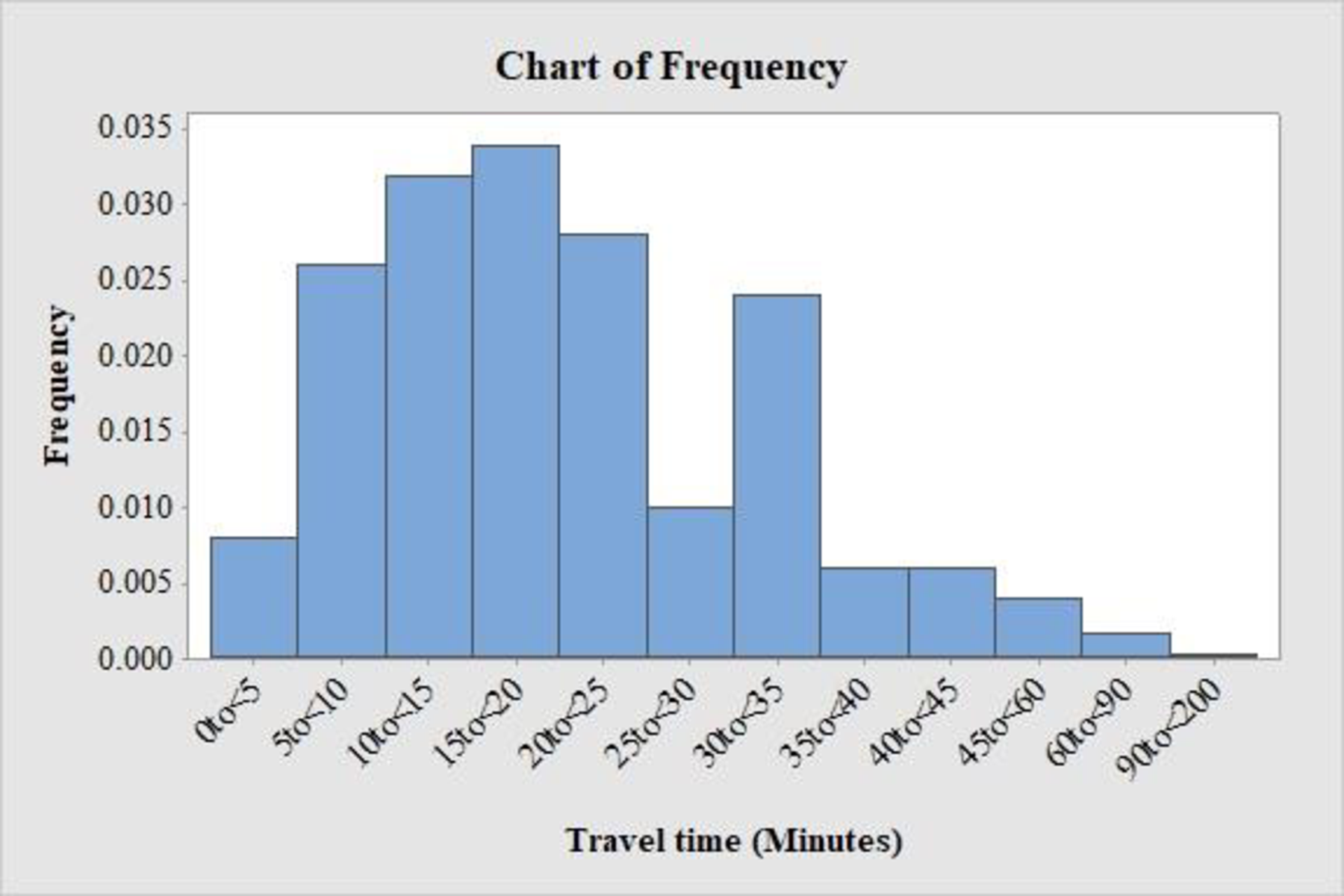
Draw a histogram for the travel time distribution.
a.
Answer to Problem 40E
The histogram for the travel time distribution is given below:
Explanation of Solution
Calculation:
The data represent the relative frequency for travel time to work for a large sample of adults who did not work at home.
Software procedure:
Step-by-step procedure to obtain the width using MINITAB software:
- Choose Calc > Calculator.
- Enter the column of width under Store result in variable.
- Enter the formula ‘Upper’-‘Lower’ under Expression.
- Click OK.
The
Step-by-step procedure to obtain the density using MINITAB software:
- Choose Calc > Calculator.
- Enter the column of Frequency under Store result in variable.
- Enter the formula ‘Frequency’/‘width’ under Expression.
- Click OK.
The density is stored in the column “Frequency”.
Step by step procedure to draw the relative frequency histogram using MINITAB software:
- Select Graph > Bar chart.
- In Bars represent select Values from a table.
- In One column of values select Simple.
- Enter Frequency in Graph variables.
- Enter Travel Time (Minutes) in categorical variable.
- Select OK.
- Click on the axis of the graph and in Gap between clusters enter 0.
Thus, the histogram for travel time is obtained.
b.
Delineate the features, such as center, shape, and variability of the histogram from Part (a).
b.
Explanation of Solution
From the histogram, it is observed that the distribution of travel time is slightly positively skewed with a single maximum frequency density, that is, a single
c.
Explain whether it is appropriate to use the
c.
Answer to Problem 40E
No, it is not appropriate to use empirical rule to make statements about the travel time distribution.
Explanation of Solution
By observing the histogram, the travel time data are skewed right. However, the empirical rule is applicable for data that are distributed normally, which is bell-shaped and symmetric.
Therefore, in this context, it is not appropriate to use the empirical rule to make the statements about the travel time distribution.
d.
Elucidate the reason why the travel time distribution could not be well approximated by a normal curve.
d.
Explanation of Solution
It is given that the approximate mean and standard deviation for the travel time distribution are 27 minutes and 24 minutes, respectively.
The observation of the travel time should not be negative. In general, the travel time begins from 0.
If the distribution of the travel time is approximately normal, then the percentage of the travel time that fall below 0 is obtained as given below:
Use the standard normal probabilities (cumulative z-curve area) table to find the z-value:
Procedure:
For z at –1.12:
- Locate –1.1 in the left column of the table.
- Obtain the value in the corresponding row below 0.02.
That is,
Therefore, the percentage of the travel time that fall below 0 is 13.14% that is not possible.
Hence, the distribution of the travel time cannot be approximated by the normal curve.
e.
Find the percentage of travel time between 0 and 75 minutes using Chebyshev’s rule.
Obtain the percentage of travel time between 0 and 47 minutes using Chebyshev’s rule.
e.
Answer to Problem 40E
The percentage of travel time between 0 and 75 minutes is at least 75%.
The percentage of travel time between 0 and 47 minutes is at least 21%.
Explanation of Solution
Calculation:
The approximate mean and standard deviation for the travel time distribution are 27 minutes and 24 minutes, respectively.
The values at 2 standard deviations away from the mean is obtained as follows:
The observation of the travel time should not be negative. Therefore, the travel time that begins at –21 minutes lies in 2 standard deviation below the mean that is not possible. Travel time 75 minutes lies 2 standard deviations above from the mean.
Chebyshev’s rule:
For any number k, where
The z-score gives the number of standard deviations that an observation of 75 minutes is away from the mean. Here, the z-scores for 0 minutes and 75 minutes are –2 and 2, respectively. Thus, these observations of time are 2 standard deviations from the mean that is
(i).
The percentage of travel time between 0 and 75 minutes is obtained as given below:
Use Chebyshev’s rule as follows:
In this context, at least 0.75 proportion of observations lie within 2 standard deviations of the mean.
Therefore, the percentage of travel time between 0 and 75 minutes is 75%.
(ii).
A travel time of 47 minutes is
A travel time of 0 minutes is
Since 1.125 is larger than 0.833, these observations of time are 1.125 standard deviations from the mean that is
The percentage of the travel times between 0 and 47 minutes is obtained as given below:
Use Chebyshev’s rule as follows:
Thus, the percentage of the travel time between 0 and 47 minutes is 21%.
f.
Explain the way why the statements in Part (e) agree with the actual percentage for the travel time distribution.
f.
Explanation of Solution
Calculation:
The actual percentage of travel time between 0 and 75 minutes is obtained as given below:
Therefore, the actual percentage of travel time between 0 and 75 minutes is approximately 95.5% and differs a lot from the percentage obtained using Chebyshev’s rule.
The actual percentage of travel times between 0 and 47 minutes is obtained as given below:
Therefore, the actual percentage of travel time between 0 and 47 minutes is approximately 90% and differs a lot from the percentage obtained using Chebyshev’s rule.
Want to see more full solutions like this?
Chapter 4 Solutions
INTRO.TO STATS.+DATA ANALYS. W/WEBASSI


- Spacers are manufactured to the mean dimension and tolerance shown in Figure 29-12. An inspector measures 10 spacers and records the following thicknesses: 0.372" 0.376" 0.379" 0.375" 0.370" 0.373" 0.377" 0.378" 0.371" 0.380" Which spacers are defective (above the maximum limit or below the minimum limit)? All dimensions are in inches.arrow_forwardTwo quality control technicians measured the surface finish of a metal part, obtaining the data in the table below. Assume that the measurements are normally distributed.arrow_forwardFor a variable with a density curve, what is the relationship between the percentage of all possible observations of the variable that lie within any specified range and the corresponding area under its density curve?arrow_forward
- 1. Consider a population consisting of the following five values, which represent the number of DVD rentalsduring the academic year for each of five housemates:8 14 16 10 11 d. Construct a density histogram using the 25 x values. Are most of the x values near the population mean? Do the x values differ a lot from sample to sample, or do they tend to be similar?arrow_forwardThe department of zoology at the Virginia Polytechnic Institute and State University carried out a study to determine if there is a significant difference in the density of organisms in two different stations located in Cedar Run, a secondary river that is located in the river basin. Roanoke. Drainage from a sewage treatment plant and overflow from the Federal Mogul Corporation sedimentation pond enter the flow near the source of the river. The following data give the density measurements, in numbers of organisms per square meter, at the two different collecting stations. Number of organisms per square meter Station 1 Station 2 5030 2800 13700 4670 10730 6890 11400 7720 860 7030 2200 7330 4250 2810 15040 1330 4980 3320 11910 1230 8130 2130 26850 2190 17660 22800 1130 1690 With a significance level of 0.05, can we conclude that the densities are the same in the two…arrow_forward
 Mathematics For Machine TechnologyAdvanced MathISBN:9781337798310Author:Peterson, John.Publisher:Cengage Learning,