
Bundle: Managerial Economics, Loose-leaf Version, 14th + MindTap Economics, 1 term (6 months) Printed Access Card
14th Edition
ISBN: 9781337127325
Author: MCGUIGAN
Publisher: CENGAGE L
expand_more
expand_more
format_list_bulleted
Videos
Textbook Question
Chapter 5, Problem 1.6CE
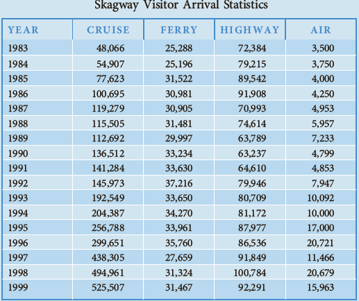
Estimate the double-log (log linear) time trend model for log cruise ship arrivals against log time. Estimate a linear time trend model of cruise ship arrivals against time. Calculate the root mean square error between the predicted and actual value of cruise ship arrivals. Is the root mean square error greater for the double log non-linear time trend model or for the linear time trend model?
Expert Solution & Answer
Want to see the full answer?
Check out a sample textbook solution
Students have asked these similar questions
Year
Quarter
Revenue
Q1
4.80
Q2
4.56
2015
Q3
4.88
Q4
4.91
Q1
5.37
Q2
4.99
2016
Q3
5.24
Q4
5.71
Q1
5.73
Q2
5.29
2017
Q3
5.66
Q4
5.70
Q1
6.07
Q2
6.03
2018
Q3
6.31
Q4
6.30
Q1
6.60
Q2
6.31
2019
Q3
6.82
Q4
6.75
Q1
7.10
Q2
6.00
2020
Q3
4.20
Q4
6.20
Historical demand for Peeps is as displayed in the table.
Month Demand
January 11
February 18
March 31
April 39
May 44
June 53
July 67
August 82
September 96
Develop forecasts from June through October using these techniques: Holt's method with alpha=0.2
and beta=0.1. For Holt's model, the level and trend for May are assumed to be 44 and
12. Judge which forecast method is the best based on MAD.
You own a restaurant near the beach. Business has been growing each
year, but obviously spikes during the summer months. A regression
produces the following equation:
M = 30,000 + 500t + 1,000S
Where M is monthly sales, t is years past 2010, and S is a dummy variable
for the summer months. If the month is June, July, or August, insert a "1"”.
If not, the value for S is zero.
What are the predicted sales for July 2020?
Enter as a value.
Chapter 5 Solutions
Bundle: Managerial Economics, Loose-leaf Version, 14th + MindTap Economics, 1 term (6 months) Printed Access Card
Ch. 5 - The forecasting staff for the Prizer Corporation...Ch. 5 - Prob. 2ECh. 5 - Metropolitan Hospital has estimated its average...Ch. 5 - Prob. 4ECh. 5 - A firm experienced the demand shown in the...Ch. 5 - The economic analysis division of Mapco...Ch. 5 - The Questor Corporation has experienced the...Ch. 5 - Bell Greenhouses has estimated its monthly demand...Ch. 5 - Savings-Mart (a chain of discount department...Ch. 5 - Prob. 1.1CE
Ch. 5 - Plot the logarithm of arrivals for each...Ch. 5 - Logarithms are especially useful for comparing...Ch. 5 - Prob. 1.4CECh. 5 - In attempting to formulate a model of the...Ch. 5 - Estimate the double-log (log linear) time trend...Ch. 5 - Prob. 2.1CECh. 5 - Prob. 3.1CECh. 5 - Prob. 3.2CECh. 5 - Prob. 3.3CE
Knowledge Booster


Learn more about
Need a deep-dive on the concept behind this application? Look no further. Learn more about this topic, economics and related others by exploring similar questions and additional content below.Similar questions
- Question 3 The number of tons of brake assemblies received at an auto parts distribution center last month was 625. The forecast tonnage was 650 for last month. The company uses a simple exponential smoothing model with a smoothing constant of 0.46 to develop its forecasts. What will be the company's forecast for the next month? Add your answerarrow_forwardTrend is oscillating pattern of increase or decrease in demand over a period of time. Select one: True Falsearrow_forwardPlot the logarithm of arrivals for each transportation mode against time, all on the same graph. Which now appears to be growing the fastest?arrow_forward
- Use simple exponential smoothing with a = 0.6 to forecast the tire sales for September through December. Assume that the forecast for August was for 46 sets of tires. Do your forecasts seem to be biased? Why or why not? Month Sales August 53 September35 October 48 November 40arrow_forwardA local moving company has collected data on the number of moves they have been asked to perform over the past two years. Moving is highly seasonal, so the owner/operator, who is both burly and highly educated, decides to apply the multiplicative seasonal method to forecast the number of customers for the coming year. The equation for the trend line of yearly sales is Ft = 16 + 60t. Please forecast demand for each quarter in Year 3. (Round the forecasts to whole numbers and show all calculations). Complete the table below and forecast the sales of Year 3 by quarter. Year 1 Year 2 Year 3 Quarter Demand Seasonal Index Quarter Demand Seasonal Index Average Seasonal Index Forecast 1 20 1 27 2 40 2 45 3 45 3 55 4 31 4 41 Total Averagearrow_forwardCalculate the percentage change of the variable in each of the following cases. Then calculate the percentage change if the movement is occurring in the opposite direction, with what was the final value now the initial value and vice versa. Now calculate a comparable percentage change using the average of the initial and ending values. Express all three changes in absolute value form without positive or negative signs and as whole numbers (i.e. 67%, not 66.6%). a. A fast-food restaurant, which originally sold hamburgers at a price of $1, increases their price to $2. The absolute value of this percentage change is %, and the absolute value of the percentage change calculated using the average of the two values is 0.5 %, the absolute value of the percentage change in the opposite direction is | %. b. The number of autos sold monthly at a car dealership drops from 150 to 50. The absolute value of this percentage change is %, and the absolute value of the percentage change calculated using…arrow_forward
- A researcher has a sample of 6 annual observations {94, 104, 102, 99, 111 and 107} for the CPI in country Z for the period 2015 to 2020, and wants to forecast CPI for the years 2021, 2022 and 2023. The researcher uses 3 different forecasting models: A, B and C. Model A is an AR(1) model with no drift and with an estimated autoregressive coefficient = 0.7. Model B is a MA(1) model with no constant and with an estimated MA coefficient = -0.4 (note the minus !). Model C is a random walk model with no drift. The error terms over the 2015-2020 period were estimated to have the values: {3, -1, 2, 4, -3, 1}. a. Compute the 2021, 2022 and 2023 forecasted values for the consumer price index based on the three models. Show the formulas and the details of your calculations, and explain all the related symbols. b. Suppose that the actual values of the CPI over the 2021, 2022 and 2023 were {108, 114, 105}. Calculate the Root mean square error of the three model forecasts over the 2021-2023…arrow_forwardCalculate the percentage change of the variable in each of the following cases. Then calculate the percentage change if the movement is occurring in the opposite direction, with what was the final value now the initial value and vice versa. Now calculate a comparable percentage change using the average of the initial and ending values. Express all three changes in absolute value form without positive or negative signs and as whole numbers (i.e. 67%, not 66.6%). a. A fast-food restaurant, which originally sold hamburgers at a price of $5, increases their price to $6. The absolute value of this percentage change is %, and the absolute value of the percentage change calculated using the average of the two values is %, the absolute value of the percentage change in the opposite direction is %. b. The number of autos sold monthly at a car dealership drops from 400 to 300. The absolute value of this percentage change is %, the absolute value of the percentage change in the opposite direction…arrow_forwardwhich sentences are correct? 1.Decomposition methods assume that the actual time series value at period t is a function of three components: trend, seasonal, and irregular. 2.Dummy variables can be used to deal with categorical independent variables in a multiple regression model. 3.If a time series exhibits a linear trend, the method of least squares may be used to determine a trend line (projection) for future forecasts. 4.Time series decomposition can be used to separate or decompose a time series into seasonal, trend, and irregular (error) components. 5.A variety of nonlinear functions can be used to develop an estimate of the trend in a time series, including quadratic trend equation and exponential trend equation. 6.Hypothesis Testing about the variances of Two Populations apply with F test Statistic. 7.Hypothesis Testing about the variances of One Populations apply with Chi test Statistic. 8.Hypothesis Testing about the variances of One Populations apply with F test Statistic.…arrow_forward
- X(t) is a wide sense stationary stochastic process with autocorrelation function sin(271000r) R„(T)=10- 271000r The process Y(t) is a version of X(t) delayed by 50 micro seconds. {Y(t) = X(t - t0)} (a) Derive the autocorrelation function of Y (t). (b) Derive the cross-correlation function of X(t) and Y (t). (c) Are X(t) and Y (t) jointly wide sense stationary? IUnloaded File Detailsarrow_forwardA manager uses a trend equation plus quarterly relatives to predict demand. Quarter relatives are SR1 = 0.9, SR2 = 0.95, SR3 = 1.05, and SR4 = 1.1. The trend equation is: Ft = 11 + 3t. Over the past nine quarters, demand has been as follows: %3D Period, t: 1 4 7 8 9. Demand: 15 17 20 23 25 29 34 36 39 Click here for the Excel Data File Compute the MAD and tracking signal for each period. (Negative values should be indicated by a minus sign. Round your intermediate calculations and final answers to 3 decimal places.) Period, t Demand MAD Tracking signal 1 15 2 17 3 20 4 23 25 6. 29 7 34 36 39 LOarrow_forwardWhat is the index formulation used for?arrow_forward
arrow_back_ios
SEE MORE QUESTIONS
arrow_forward_ios
Recommended textbooks for you
 Managerial Economics: Applications, Strategies an...EconomicsISBN:9781305506381Author:James R. McGuigan, R. Charles Moyer, Frederick H.deB. HarrisPublisher:Cengage Learning
Managerial Economics: Applications, Strategies an...
Economics
ISBN:9781305506381
Author:James R. McGuigan, R. Charles Moyer, Frederick H.deB. Harris
Publisher:Cengage Learning
Forecasting: Exponential Smoothing, MSE; Author: Joshua Emmanuel;https://www.youtube.com/watch?v=k_HN0wOKDd0;License: Standard Youtube License