
Videos
An accurate assessment of oxygen consumption provides important information for determining energy expenditure requirements for physically demanding tasks. The paper “Oxygen Consumption During Fire Suppression: Error of Heart Rate Estimation” (Ergonomics [1991]: 1469–1474) reported on a study in which x = Oxygen consumption (in milliliters per kilogram per minute) during a treadmill test was determined for a sample of 10 firefighters. Then y = Oxygen consumption at a comparable heart rate was measured for each of the 10 individuals while they performed a fire-suppression simulation. This resulted in the following data and

- a. Does the scatterplot suggest an approximate linear relationship?
- b. The investigators fit a least-squares line. The resulting Minitab output is given in the following:
The regression equation is firecon = 211. 4 + 1. 09 treadcon
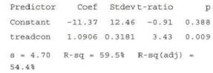
Predict fire-simulation consumption when treadmill consumption is 40.
- c. How effectively does a straight line summarize the relationship?
- d. Delete the first observation, (51.3, 49.3), and calculate the new equation of the least-squares line and the value of r2. What do you conclude? (Hint: For the original data, Σx = 388.8, Σy = 310 .3, Σx2 = 15,338.54, Σxy = 12,306.58, and Σy2 = 10,072.41.)
a.
Discuss whether the scatterplot indicates an approximate linear relationship.
Answer to Problem 66CR
No, the scatterplot does not indicate an approximate linear relationship.
Explanation of Solution
The data relates the oxygen consumption (milliliters per kilogram per minute) of 10 firefighters during a fire-suppression simulation, y to that during a treadmill test, x. The scatterplot between the two variables is given.
Denote the estimated response variable as
A careful inspection of the given scatterplot shows that the points do not fall on a straight line. Rather, the points are scattered almost in a random manner, without showing any pattern in particular. However, there is one extreme point, which is far away from the remaining points. This extreme point appears to provide an impression that there might be a linear relationship between the two variables. Once this point is ignored, it is clear that no such relationship can be determined.
Thus, the scatterplot does not indicate an approximate linear relationship.
b.
Predict the fire-simulation oxygen consumption, if the treadmill oxygen consumption is 40.
Answer to Problem 66CR
The fire-simulation oxygen consumption, when the treadmill oxygen consumption is 40 is 32.254 milliliters per kilogram per minute.
Explanation of Solution
Calculation:
The MINITAB output for the fitting of a least-squares regression line to the given data is given.
In the given output, the column of “Coef” gives the coefficients corresponding to the variables given in the column of “Predictor”. The term “Constant” under the column of ‘Predictor’ gives the intercept of the equation; the term “treadcon” denotes the oxygen consumption of during the treadmill test, x.
Using the values in the output, the equation of the least-squares regression line is
For a treadmill oxygen consumption of 40 milliliters per kilogram per minute,
Thus, the fire-simulation oxygen consumption, when the treadmill oxygen consumption is 40 is 32.254 milliliters per kilogram per minute.
c.
Explain the effectivity of the straight line to summarize the relationship between the variables.
Explanation of Solution
In the given output, the value of
Now,
Thus, it can be interpreted that the oxygen consumption during the treadmill test can predict about 59.5% of the variability in the oxygen consumption during the fire-suppression simulation.
This suggests that the straight line is moderately effective in summarizing the relationship between the variables.
d.
Find the equation of the least-squares line and the value of
Answer to Problem 66CR
The equation of the least-squares line after deleting the first observation, (51.3, 49.3) is
The value of
Explanation of Solution
Calculation:
It is given that, for the original data set,
For the first observation,
Now, the lest-squares regression line is of the form:
Using this formula and the values obtained above, b and a are respectively obtained as follows:
Now,
Thus,
Using the values of a and b obtained above, the equation of the least-squares line after deleting the first observation, (51.3, 49.3) is
Now, it is known that the slope for the least-squares regression of y on x, that is, b can be given by the formula:
Now, it can be shown that:
Similarly,
Thus,
Using the values obtained above, the value of r can be calculated as follows:
It is known that
Hence, the value of
Now,
Now,
Thus, it can be interpreted that the oxygen consumption during the treadmill test can predict about 2% of the variability in the oxygen consumption during the fire-suppression simulation, which is a very low percentage.
Thus, the model 9is not a very good fit for the data.
Want to see more full solutions like this?
Chapter 5 Solutions
INTRO.TO STATS.+DATA ANALYS. W/WEBASSI
Additional Math Textbook Solutions
Statistics for Business & Economics, Revised (MindTap Course List)
Elementary Statistics
Basic Business Statistics, Student Value Edition
Introductory Statistics (2nd Edition)
Elementary Statistics: A Step By Step Approach
Essentials of Statistics, Books a la Carte Edition (5th Edition)


- The article “Withdrawal Strength of Threaded Nails” (D. Rammer, S. Winistorfer, and D. Bender, Journal of Structural Engineering 2001:442–449) describes an experiment comparing the ultimate withdrawal strengths (in N/mm) for several types of nails. For an annularly threaded nail with shank diameter 3.76 mm driven into spruce-pine-fir lumber, the ultimate withdrawal strength was modeled as lognormal with μ = 3.82 and σ = 0.219. For a helically threaded nail under the same conditions, the strength was modeled as lognormal with μ = 3.47 and σ = 0.272. a) What is the mean withdrawal strength for annularly threaded nails? b) What is the mean withdrawal strength for helically threaded nails? c) For which type of nail is it more probable that the withdrawal strength will be greater than 50 N/mm? d) What is the probability that a helically threaded nail will have a greater withdrawal strength than the median for annularly threaded nails? e) An experiment is performed in which withdrawal…arrow_forwardLactation promotes a temporary loss of bone mass to provide adequate amounts of calcium for milk production. The paper “Bone Mass Is Recovered from Lactation to Postweaning in Adolescent Mothers with Low Calcium Intakes” (Amer. J. of Clinical Nutr., 2004: 1322–1326) gave the following data on total body bone mineral content (TBBMC) (g) for a sample both during lactation (L) and in the postweaning period (P). SubjectL 1928 2549 2825 1924 1628 2175 2114 2621 1843 2541P 2126 2885 2895 1942 1750 2184 2164 2626 2006 2627 Does the data suggest that true average total body bone mineral content during postweaning exceeds that during lactation by more than 25 g? State and test the appropriate hypotheses using a significance level of .05.arrow_forwardA deficiency of the trace element selenium in the diet can negatively impact growth, immunity, muscle and neuromuscular function, and fertility. The introduction of selenium supplements to dairy cows is justified when pastures have low selenium levels. Authors of the article “Effects of Short-Term Supplementation with Selenised Yeast on Milk Production and Composition of Lactating Cows” (Australian J. of Dairy Tech., 2004: 199–203) supplied the following data on milk selenium concentration (mg/L) for a sample of cows given a selenium supplement and a control sample given no supplement, both initially and after a 9-day period. Obs Init Se Init Cont Final Se Final Cont 1 11.4 9.1 138.3 9.3 2 9.6 8.7 104 8.8 3 10.1 9.7 96.4 8.8 4 8.5 10.8 89 10.1 5 10.3 10.9 88 9.6 6 10.6 10.6 103.8 8.6 7 11.8 10.1 147.3 10.4 8 9.8 12.3 97.1 12.4 9 10.9 8.8 172.6 9.3 10 10.3…arrow_forward
- J 2 RCT was conducted to evaluate efficacy and safety of drug simvastatin compared to placebo in reducing mortality and morbidity in patients with coronary heart disease. Subjects were followed up on average 5.4 years. Over the duration of the follow-up, 63 subjects died due to heart attack among 2,223 subjects in the placebo group compared to 30 deaths among 2,221 patients in the simvastatin drug group. 1. What is the Relative Risk or death from the heart attack in the simvastatin group?arrow_forwardA study was conducted to examine if children with autism spectrum disorder (ASD) had higher prenatal exposure to air pollution, specifically particulate matter < 2.5 g in diameter (PM2.5). Researchers obtained birth records of all children born in Los Angeles between 2000 and 2008 and linked these to the Department of Developmental Services records to determine if any of those subjects had been diagnosed with ASD or not. They used the birth addresses given in the birth records to determine the average daily PM2.5 for the third trimester for each child. The standard deviation for PM2.5 among ASD subjects was found to be 34.6 and for non-ASD subjects was 16.8. Assume PM2.5 is normally distributed. 4a. What was the study design? * Randomized Clinical Trial (RCT) * Case Report * Nested Case-Control Study * Case-Control Study * cross-sectional study Cohort Study 4B. What are the null and alternative hypotheses? 4c. What type of statistical test would you use to analyze the…arrow_forwardResearchers interested in lead exposure due to car exhaust sampled the blood of 52 police officers subjected to constant inhalation of automobile exhaust fumes while working traffic enforcement in a primarily urban environment. The blood samples of these officers had an average lead concentration of 124.32 µg/l and an SD of 37.74 µg/l; a previous study of individuals from a nearby suburb, with no history of exposure, found an average blood level concentration of 35 µg/l. Write down the hypotheses that would be appropriate for testing if the police officers appear to have been exposed to a higher concentration of lead. Explicitly state and check all conditions necessary for inference on these data. Test the hypothesis that the downtown police officers have a higher lead exposure than the group in the previous study. Interpret your results in context. Based on your preceding result, without performing a calculation, would a 99% confidence interval for the average blood concentration…arrow_forward
- Compare the two separate scatterplots. In particular, how do the associtation compare between women with pets vs. women without pets? Does one group have more variation in systolic blood pressure than the other? If so, for which group? Does systolic blood pressure seem higher for common ages between the two groups? If so, for which group?arrow_forwardA deficiency of the trace element selenium in the diet can negatively impact growth, immunity, muscle and neuromuscular function, and fertility. The introduction of selenium supplements to dairy cows is justified when pastures have low selenium levels. Authors of a research paper supplied the following data on milk selenium concentration (mg/L) for a sample of cows given a selenium supplement (the treatment group) and a control sample given no supplement, both initially and after a 9-day period. Initial Measurement Treatment Control 11.2 9.1 9.6 8.7 10.1 9.7 8.5 10.8 10.3 10.9 10.6 10.6 11.7 10.1 9.7 12.3 10.8 8.8 10.3 10.4 10.4 10.9 11.2 10.4 9.4 11.6 10.6 10.9 10.7 8.4 After 9 Days Treatment Control 138.3 9.3 104 8.7 96.4 8.7 89 10.1 88 9.6 103.8 8.6 147.3 10.2 97.1 12.2 172.6 9.3 146.3 9.5 99 8.2 122.3 8.9 103 12.5 117.8 9.1 121.5 93 (a) Use the given data for the treatment group to determine if there…arrow_forwardA deficiency of the trace element selenium in the diet can negatively impact growth, immunity, muscle and neuromuscular function, and fertility. The introduction of selenium supplements to dairy cows is justified when pastures have low selenium levels. Authors of a research paper supplied the following data on milk selenium concentration (mg/L) for a sample of cows given a selenium supplement (the treatment group) and a control sample given no supplement, both initially and after a 9-day period. Initial Measurement Treatment Control 11.3 9.1 9.7 8.7 10.1 9.7 8.5 10.8 10.4 10.9 10.7 10.6 11.8 10.1 9.8 12.3 10.6 8.8 10.4 10.4 10.2 10.9 11.3 10.4 9.2 11.6 10.7 10.9 10.8 8.2 After 9 Days Treatment Control 138.3 9.4 104 8.8 96.4 8.8 89 10.1 88 9.7 103.8 8.7 147.3 10.3 97.1 12.3 172.6 9.4 146.3 9.5 99 8.3 122.3 8.9 103 12.5 117.8 9.1 121.5 93 (a) Use the given data for the treatment group to determine if…arrow_forward
- A deficiency of the trace element selenium in the diet can negatively impact growth, immunity, muscle and neuromuscular function, and fertility. The introduction of selenium supplements to dairy cows is justified when pastures have low selenium levels. Authors of a research paper supplied the following data on milk selenium concentration (mg/L) for a sample of cows given a selenium supplement (the treatment group) and a control sample given no supplement, both initially and after a 9-day period. Initial Measurement Treatment Control 11.4 9.1 9.6 8.7 10.1 9.7 8.5 10.8 10.2 10.9 10.6 10.6 11.9 10.1 9.9 12.3 10.7 8.8 10.2 10.4 10.3 10.9 11.4 10.4 9.3 11.6 10.6 10.9 10.9 8.3 After 9 Days Treatment Control 138.3 9.2 104 8.9 96.4 8.9 89 10.1 88 9.6 103.8 8.6 147.3 10.4 97.1 12.4 172.6 9.2 146.3 9.5 99 8.4 122.3 8.8 103 12.5 117.8 9.1 121.5 93 (a) Use the given data for the treatment group to determine if…arrow_forwardSuppose a researcher is interested inthe effectiveness in a new childhood exercise program implemented in a SRS of schools across a particular county. In order to test the hypothesis that the new program decreases BMI (Kg/m2), the researcher takes a SRS of children from schools where the program is employed and a SRS from schools that do not employ the program and compares the results. Assume the following table represents the SRSs of students and their BMIs. Student intervention group BMI (kg/m2) Student control group BMI (kg/m2) A 18.6 A 21.6 B 18.2 B 18.9 C 19.5 C 19.4 D 18.9 D 22.6 E 24.1 F 23.6 A) Assuming that all the necessary conditions are met (normality, independence, etc.) carry out the appropriate statistical test to determine if the new exercise program is effective. Use an alpha level of 0.05. Do not assume equal variances.B) Construct a 95% confidence interval about your estimate for the average difference in BMI between the groups.arrow_forwardThe Road Department is trying to see whether they should buy road treatments ( in tons) for storms based on the number of inches of snow for each recorded. Use Pearson r at alpha- 0.05 to test the hypothesis. ILLUSTRATE THE NORMAL CURVE inches in snow 1.5 1.7 3.7 2.8 4.6 2.4 3.1 2.9 3.6 4.2 3.1 number of tons 805 905 1235 1000 1302 998 1102 1305 1456 1600 1005arrow_forward
 MATLAB: An Introduction with ApplicationsStatisticsISBN:9781119256830Author:Amos GilatPublisher:John Wiley & Sons Inc
 Probability and Statistics for Engineering and th...StatisticsISBN:9781305251809Author:Jay L. DevorePublisher:Cengage Learning
 Statistics for The Behavioral Sciences (MindTap C...StatisticsISBN:9781305504912Author:Frederick J Gravetter, Larry B. WallnauPublisher:Cengage Learning
 Elementary Statistics: Picturing the World (7th E...StatisticsISBN:9780134683416Author:Ron Larson, Betsy FarberPublisher:PEARSON
 The Basic Practice of StatisticsStatisticsISBN:9781319042578Author:David S. Moore, William I. Notz, Michael A. FlignerPublisher:W. H. Freeman
 Introduction to the Practice of StatisticsStatisticsISBN:9781319013387Author:David S. Moore, George P. McCabe, Bruce A. CraigPublisher:W. H. Freeman