
Concept explainers
Videos
(a)
To find: The probability of the sample proportion of heads between 0.4 and 0.6 by using normal to the binomial approximate.
(a)
Answer to Problem 43UYK
Solution: The probability is 0.9953.
Explanation of Solution
Calculation: When a coin is tossed, there are two possible outcomes, “heads” or “tails.” The probability of the heads coming up in a coin toss is calculated as:
The average of the sample proportion is calculated as:
The standard deviation of the sample proportion is calculated as:
Hence, the average value and standard deviation are 0.5 and 0.03536, respectively. Now, calculate the z-score,
The lower bound is
Calculate the z-score for the upper bound
Now, Excel is used to calculate the left tailed areas between the z scores. Use the formula
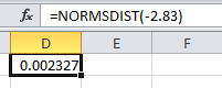
Use the formula
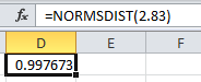
The area between them is calculated by subtracting the above values as:
Hence, the probability is 0.9953.
(b)
To find: The probability of the sample proportion of heads between 0.45 and 0.55 by using normal to the binomial approximate.
(b)
Answer to Problem 43UYK
Solution: The probability is 0.8426.
Explanation of Solution
Calculation: When a coin is tossed, there are two possible outcomes, “heads” or “tails.”
The probability of the heads coming up in a coin toss is calculated as:
The average of the sample proportion is calculated as:
The standard deviation of the sample proportion is calculated as:
Hence, the average value and standard deviation are 0.5 and 0.03536 respectively. Now, calculate the z-score,
The lower bound is
Calculate the z-score for the upper bound
Now, Excel is used to calculate the left tailed areas between the z scores. Use the formula
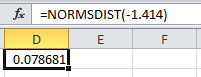
Use the formula
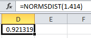
The area between them is calculated by subtracting the above values as:
Hence, the probability is 0.8426
Want to see more full solutions like this?
Chapter 5 Solutions
INTRO.TO PRACTICE STATISTICS-ACCESS


 MATLAB: An Introduction with ApplicationsStatisticsISBN:9781119256830Author:Amos GilatPublisher:John Wiley & Sons Inc
 Probability and Statistics for Engineering and th...StatisticsISBN:9781305251809Author:Jay L. DevorePublisher:Cengage Learning
 Statistics for The Behavioral Sciences (MindTap C...StatisticsISBN:9781305504912Author:Frederick J Gravetter, Larry B. WallnauPublisher:Cengage Learning
 Elementary Statistics: Picturing the World (7th E...StatisticsISBN:9780134683416Author:Ron Larson, Betsy FarberPublisher:PEARSON
 The Basic Practice of StatisticsStatisticsISBN:9781319042578Author:David S. Moore, William I. Notz, Michael A. FlignerPublisher:W. H. Freeman
 Introduction to the Practice of StatisticsStatisticsISBN:9781319013387Author:David S. Moore, George P. McCabe, Bruce A. CraigPublisher:W. H. Freeman