Concept explainers
Videos
Specialty Toys
Specialty Toys, Inc., sells a variety of new and innovative children’s toys. Management learned that the preholiday season is the best time to introduce a new toy, because many families use this time to look for new ideas for December holiday gifts. When Specialty discovers a new toy with good market potential, it chooses an October market entry date.
In order to get toys in its stores by October, Specialty places one-time orders with its manufacturers in June or July of each year. Demand for children’s toys can be highly volatile. If a new toy catches on, a sense of shortage in the marketplace often increases the demand to high levels and large profits can be realized. However, new toys can also flop, leaving Specialty stuck with high levels of inventory that must be sold at reduced prices. The most important question the company faces is deciding how many units of a new toy should be purchased to meet anticipated sales demand. If too few are purchased, sales will be lost; if too many are purchased, profits will be reduced because of low prices realized in clearance sales.
For the coming season, Specialty plans to introduce a new product called Weather Teddy. This variation of a talking teddy bear is made by a company in Taiwan. When a child presses Teddy’s hand, the bear begins to talk. A built-in barometer selects one of five responses that predict the weather conditions. The responses
As with other products, Specialty faces the decision of how many Weather Teddy units to order for the coming holiday season. Members of the management team suggested order quantities of 15,000, 18,000, 24,000, or 28,000 units. The wide range of order quantities suggested indicates considerable disagreement concerning the market potential. The product management team asks you for an analysis of the stock-out probabilities for various order quantities, an estimate of the profit potential, and to help make an order quantity recommendation. Specialty expects to sell Weather Teddy for $24 based on a cost of $16 per unit. If inventory remains after the holiday season, Specialty will sell all surplus inventory for $5 per unit. After reviewing the sales history of similar products, Specialty’s senior sales forecaster predicted an expected demand of 20,000 units with a .95 probability that demand would be between 10,000 units and 30,000 units. Managerial Report
Prepare a managerial report that addresses the following issues and recommends an order quantity for the Weather Teddy product.
- 1. Use the sales forecaster’s prediction to describe a
normal probability distribution that can be used to approximate the demand distribution. Sketch the distribution and show its mean and standard deviation. - 2. Compute the probability of a stock-out for the order quantities suggested by members of the management team.
- 3. Compute the projected profit for the order quantities suggested by the management team under three scenarios: worst case in which sales = 10,000 units, most likely case in which sales = 20,000 units, and best case in which sales = 30,000 units.
- 4. One of Specialty’s managers felt that the profit potential was so great that the order quantity should have a 70% chance of meeting demand and only a 30% chance of any stock-outs. What quantity would be ordered under this policy, and what is the projected profit under the three sales scenarios?
- 5. Provide your own recommendation for an order quantity and note the associated profit projections. Provide a rationale for your recommendation.
1.
Describe a normal probability distribution that can be used to approximate the demand distribution using the sales forecaster’s prediction.
Sketch the distribution and show its mean and standard deviation.
Answer to Problem 1CP
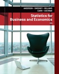
The normal distribution with a mean of 20,000 and a standard deviation of 5,102 can be used to approximate the demand distribution using the sales forecaster’s prediction.
The normal probability distribution that can be used to approximate the demand distribution is shown below:
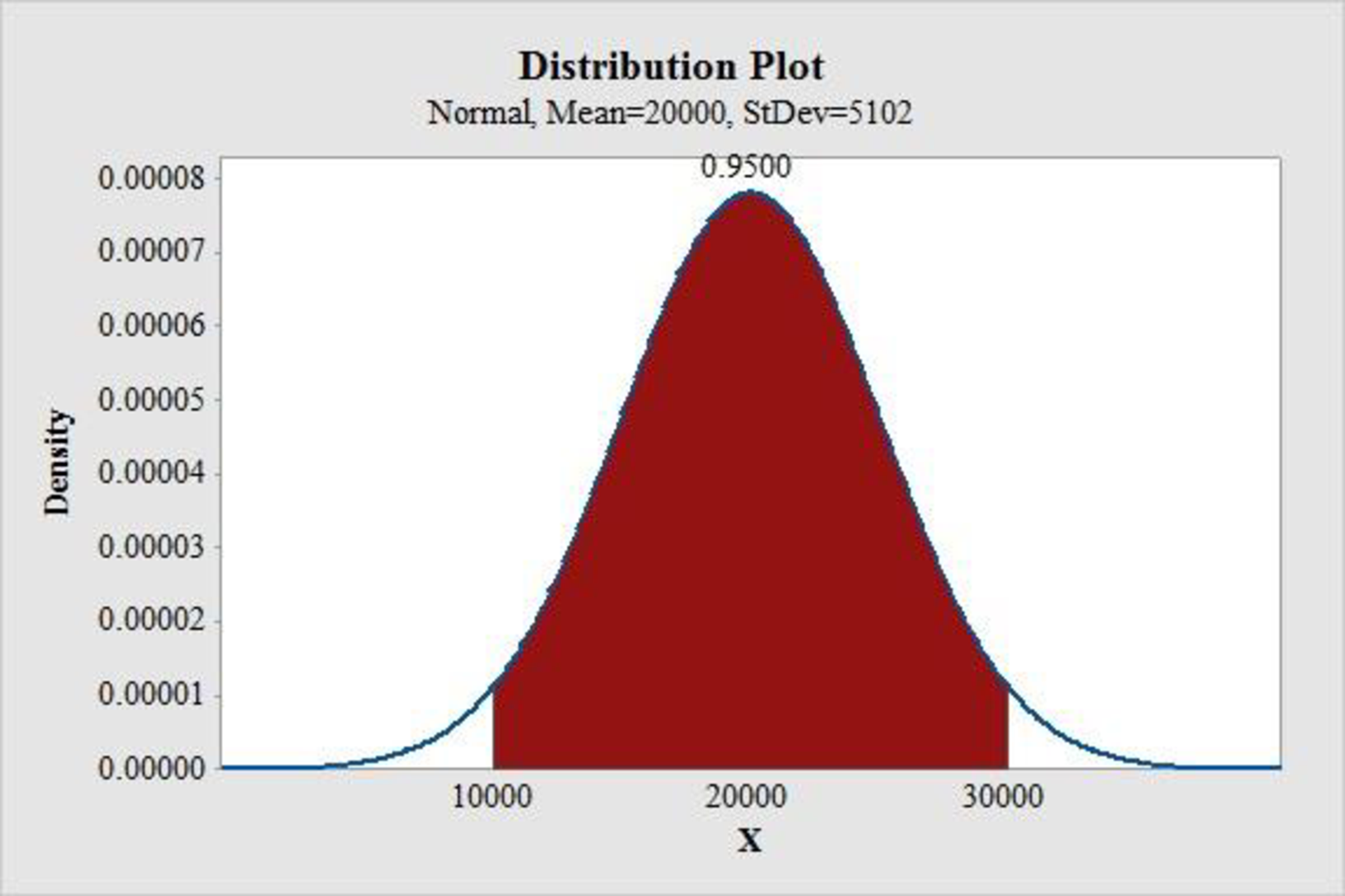
Figure (1)
Explanation of Solution
Calculation:
The order quantities suggested are 15,000, 18,000, 24,000 or 28,000 units. The Weather Teddy is expected to be sold at $24 based on a cost of $16 per unit. All surplus inventories are sold at a cost of $5 per unit. The sales forecaster’s predicted that there will be an expected demand of 20,000 units with a 0.95 probability that demand would be between 10,000 units and 30,000 units.
Define the random variable x as the demand.
From the information provided by the forecaster, demand would be between 10,000 units and 30,000 units with a 0.95 probability.
Software Procedure:
Step-by-step procedure to obtain the z-values using the MINITAB software:
- Choose Graph > Probability Distribution Plot.
- Choose View Probability > OK.
- From Distribution, choose ‘Normal’ distribution.
- Enter the Mean as 0 and Standard deviation as 1.
- Click the Shaded Area tab.
- Choose Probability and Both Tails for the region of the curve to shade.
- Enter the Probability value as 0.05.
- Click OK.
Output using the MINITAB software is given below:
From the MINITAB output the z-values are –1.96 and 1.96.
The formula for z-score is,
At
Thus, the normal distribution with a mean of 20,000 and a standard deviation of 5,102 can be used to approximate the demand distribution using the sales forecaster’s prediction.
Software Procedure:
Step-by-step procedure to draw the normal curve using the MINITAB software:
- Choose Graph > Probability Distribution Plot.
- Choose View Probability > OK.
- From Distribution, choose ‘Normal’ distribution.
- Enter the Mean as 20,000 and Standard deviation as 5,102.
- Click the Shaded Area tab.
- Choose X value and Middle area for the region of the curve to shade.
- Enter the as 0.05.
- Click OK.
The normal curve for demand is shown in figure (1).
2.
Find the probability of a stock-out for the order quantities suggested by members of the management team.
Answer to Problem 1CP
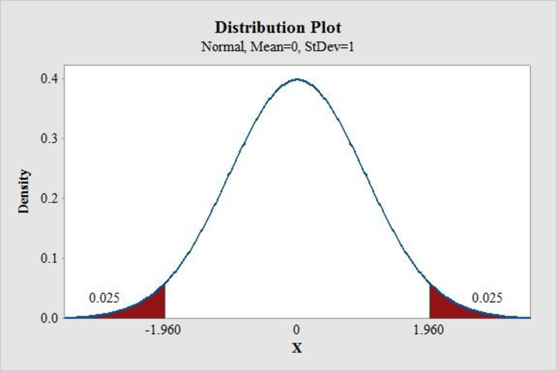
The probability of a stock-out for the order quantity of 15,000 units is 0.8365.
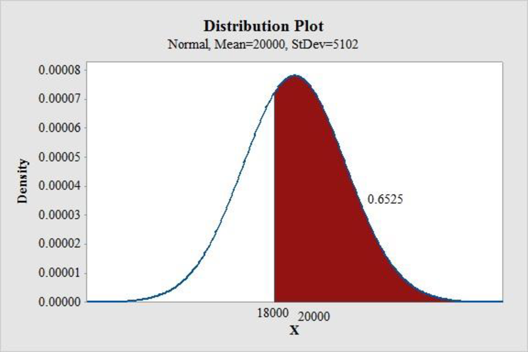
The probability of a stock-out for the order quantity of 18,000 units is 0.6525.
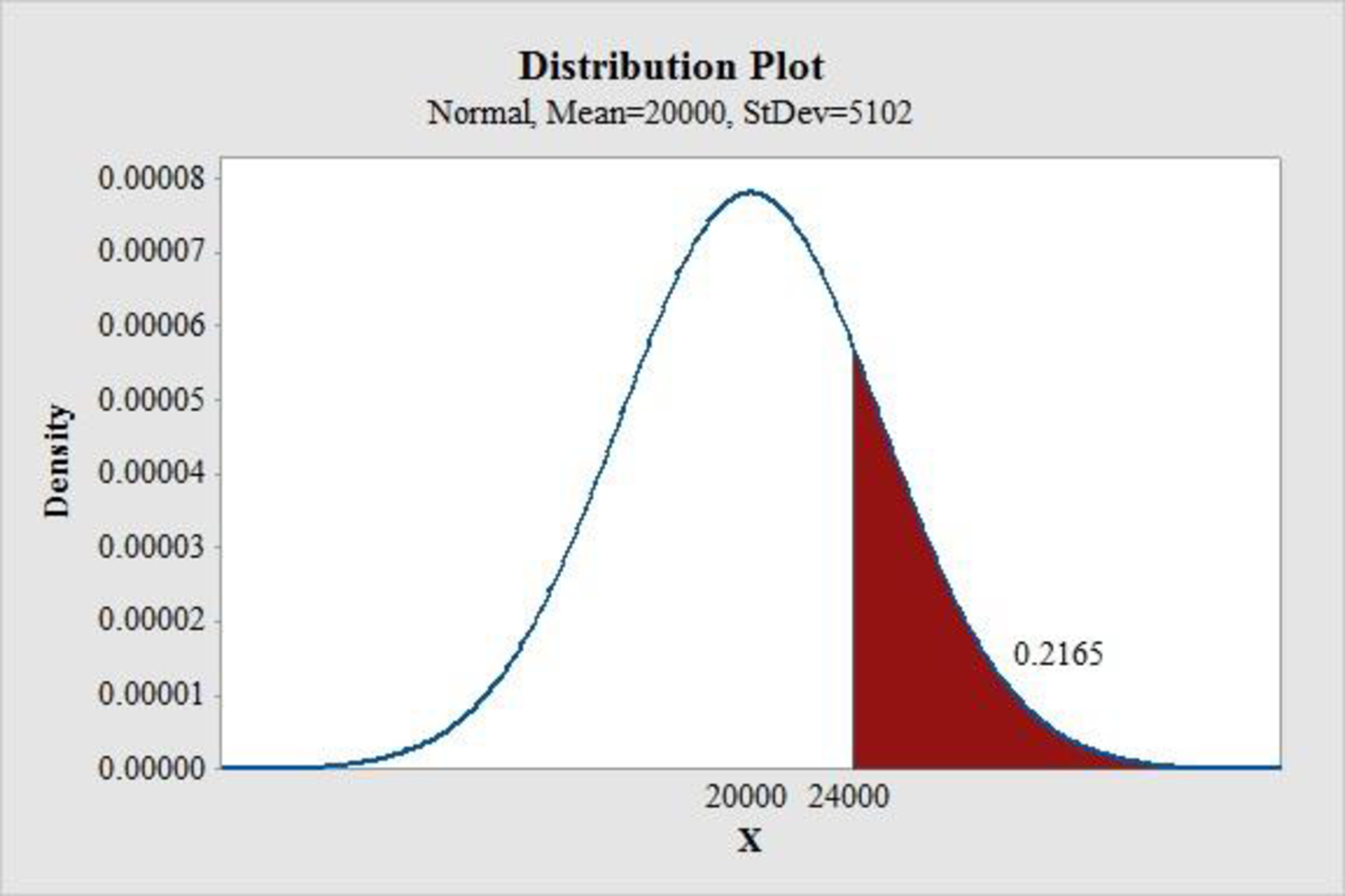
The probability of a stock-out for the order quantity of 24,000 units is 0.2165.
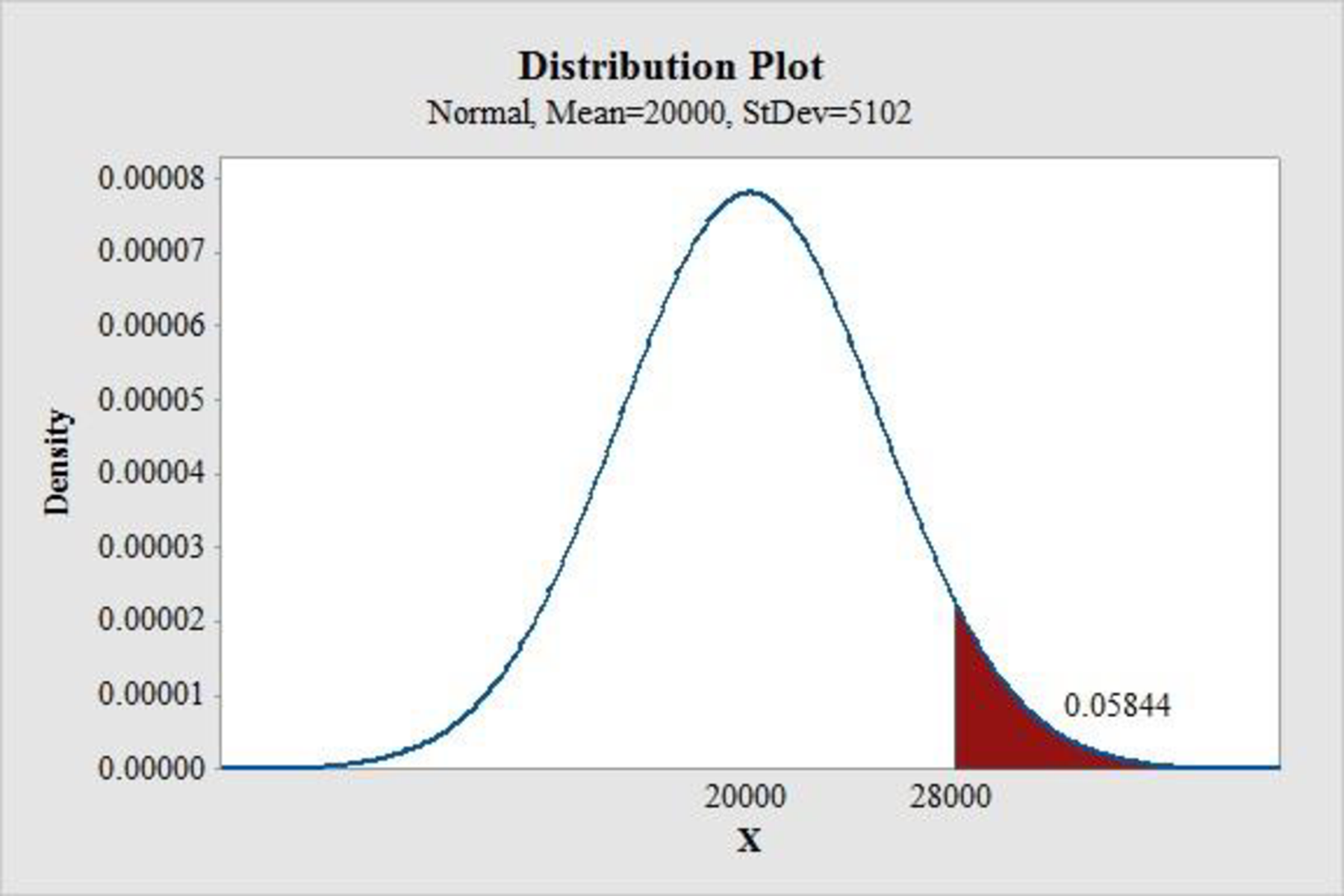
The probability of a stock-out for the order quantity of 28,000 units is 0.05844.
Explanation of Solution
Calculation:
The probability of a stock-out for the order quantity of 15,000 units is
Software Procedure:
Step-by-step procedure to obtain the probability value using the MINITAB software:
- Choose Graph > Probability Distribution Plot
- Choose View Probability > OK.
- From Distribution, choose ‘Normal’ distribution.
- Enter the Mean as 20,000 and Standard deviation as 5,102.
- Click the Shaded Area tab.
- Choose X Value and Right Tail for the region of the curve to shade.
- Enter the X value as 15,000.
- Click OK.
Output using the MINITAB software is given below:
From the MINITAB output,
Thus, the probability of a stock-out for the order quantity of 15,000 units is 0.8365.
The probability of a stock-out for the order quantity of 18,000 units is
Software Procedure:
Step-by-step procedure to obtain the probability value using the MINITAB software:
- Choose Graph > Probability Distribution Plot
- Choose View Probability > OK.
- From Distribution, choose ‘Normal’ distribution.
- Enter the Mean as 20,000 and Standard deviation as 5,102.
- Click the Shaded Area tab.
- Choose X Value and Right Tail for the region of the curve to shade.
- Enter the X value as 18,000.
- Click OK.
Output using the MINITAB software is given below:
From the MINITAB output,
Thus, the probability of a stock-out for the order quantity of 18,000 units is 0.6525.
The probability of a stock-out for the order quantity of 24,000 units is
Software Procedure:
Step-by-step procedure to obtain the probability value using the MINITAB software:
- Choose Graph > Probability Distribution Plot
- Choose View Probability > OK.
- From Distribution, choose ‘Normal’ distribution.
- Enter the Mean as 20,000 and Standard deviation as 5,102.
- Click the Shaded Area tab.
- Choose X Value and Right Tail for the region of the curve to shade.
- Enter the X value as 24,000.
- Click OK.
Output using the MINITAB software is given below:
From the MINITAB output,
Thus, the probability of a stock-out for the order quantity of 24,000 units is 0.2165.
The probability of a stock-out for the order quantity of 28,000 units is
Software Procedure:
Step-by-step procedure to obtain the probability value using the MINITAB software:
- Choose Graph > Probability Distribution Plot
- Choose View Probability > OK.
- From Distribution, choose ‘Normal’ distribution.
- Enter the Mean as 20,000 and Standard deviation as 5,102.
- Click the Shaded Area tab.
- Choose X Value and Right Tail for the region of the curve to shade.
- Enter the X value as 28,000.
- Click OK.
Output using the MINITAB software is given below:
From the MINITAB output,
Thus, the probability of a stock-out for the order quantity of 28,000 units is 0.05844.
3.
Find the projected profit for the order quantities suggested by the management team under the three scenarios.
Answer to Problem 1CP
The projected profit for the order quantities are given below:
For an order quantity of 15,000 units:
| Unit sales | Total cost ($) | At $24 | At $5 | Profit($) |
| 10,000 | 240,000 | 240,000 | 25,000 | 25,000 |
| 20,000 | 240,000 | 360,000 | 0 | 120,000 |
| 30,000 | 240,000 | 360,000 | 0 | 120,000 |
For an order quantity of 18,000 units:
| Unit sales | Total cost ($) | At $24 | At $5 | Profit($) |
| 10,000 | 288,000 | 240,000 | 40,000 | –8,000 |
| 20,000 | 288,000 | 432,000 | 0 | 144,000 |
| 30,000 | 288,000 | 432,000 | 0 | 144,000 |
For an order quantity of 24,000 units:
| Unit sales | Total cost ($) | At $24 | At $5 | Profit($) |
| 10,000 | 384,000 | 240,000 | 70,000 | –74,000 |
| 20,000 | 384,000 | 480,000 | 20,000 | 116,000 |
| 30,000 | 384,000 | 576,000 | 0 | 192,000 |
For an order quantity of 28,000 units:
| Unit sales | Total cost ($) | At $24 | At $5 | Profit($) |
| 10,000 | 448,000 | 240,000 | 90,000 | –118,000 |
| 20,000 | 448,000 | 480,000 | 40,000 | 72,000 |
| 30,000 | 448,000 | 672,000 | 0 | 224,000 |
Explanation of Solution
Calculation:
The three scenarios under consideration are, worst case in which there is a sale of 10,000 units, most likely case in which there is a sale of 20,000 units and the best case in which there is a sale of 30,000 units.
The profit projections for the order quantities under three scenarios are computed using the following table:
For an order quantity of 15,000 units:
Total cost is obtained by multiplying the cost of a unit ($16) with the order quantity.
The income at $24 is obtained by multiplying $24 with the number of units sold.
For the unit sales more than 15, 000, the income at $24 is obtained by multiplying $24 with the order quantity 15,000 units.
The income at $5 is obtained by multiplying $5 with the number of surplus units (number of units sold–order quantity).
The income at $5 will be zero for the order quantities more than 15,000 units.
The profit is obtained as shown below:
Profit obtained for a sale of 10,000 units is,
| Unit sales | Total cost ($) | At $24 | At $5 | Profit($) |
| 10,000 | 240,000 | 240,000 | 25,000 | 25,000 |
| 20,000 | 240,000 | 360,000 | 0 | 120,000 |
| 30,000 | 240,000 | 360,000 | 0 | 120,000 |
Similarly, the profit projections are obtained and are given in the following tables:
For an order quantity of 18,000 units:
| Unit sales | Total cost ($) | At $24 | At $5 | Profit($) |
| 10,000 | 288,000 | 240,000 | 40,000 | –8,000 |
| 20,000 | 288,000 | 432,000 | 0 | 144,000 |
| 30,000 | 288,000 | 432,000 | 0 | 144,000 |
For an order quantity of 24,000 units:
| Unit sales | Total cost ($) | At $24 | At $5 | Profit($) |
| 10,000 | 384,000 | 240,000 | 70,000 | –74,000 |
| 20,000 | 384,000 | 480,000 | 20,000 | 116,000 |
| 30,000 | 384,000 | 576,000 | 0 | 192,000 |
For an order quantity of 28,000 units:
| Unit sales | Total cost ($) | At $24 | At $5 | Profit($) |
| 10,000 | 448,000 | 240,000 | 90,000 | –118,000 |
| 20,000 | 448,000 | 480,000 | 40,000 | 72,000 |
| 30,000 | 448,000 | 672,000 | 0 | 224,000 |
4.
Find quantity that would be ordered under the policy and the profit at three sales scenarios.
Answer to Problem 1CP
The quantity that would be ordered under the policy is 22,675.
The profit at three sales scenarios are given in the following table:
| Unit sales | Total cost ($) | At $24 | At $5 | Profit($) |
| 10,000 | 362,800 | 240,000 | 63,375 | –59,425 |
| 20,000 | 362,800 | 480,000 | 13,375 | 130,575 |
| 30,000 | 362,800 | 544,200 | 0 | 181,400 |
Explanation of Solution
Calculation:
The order quantity should have a 70% chance of meeting demand and only a 30% chance of any stock outs. That is the order quantity that cuts off an area of 0.70 in the lower tail of the normal curve for demand.
Software Procedure:
Step-by-step procedure to obtain the x value using the MINITAB software:
- Choose Graph > Probability Distribution Plot.
- Choose View Probability > OK.
- From Distribution, choose ‘Normal’ distribution.
- Enter the Mean as 20,000 and Standard deviation as 5,102.
- Click the Shaded Area tab.
- Choose Probability Value and left tail for the region of the curve to shade.
- Enter the Probability value as 0.70.
- Click OK.
Output using the MINITAB software is given below:
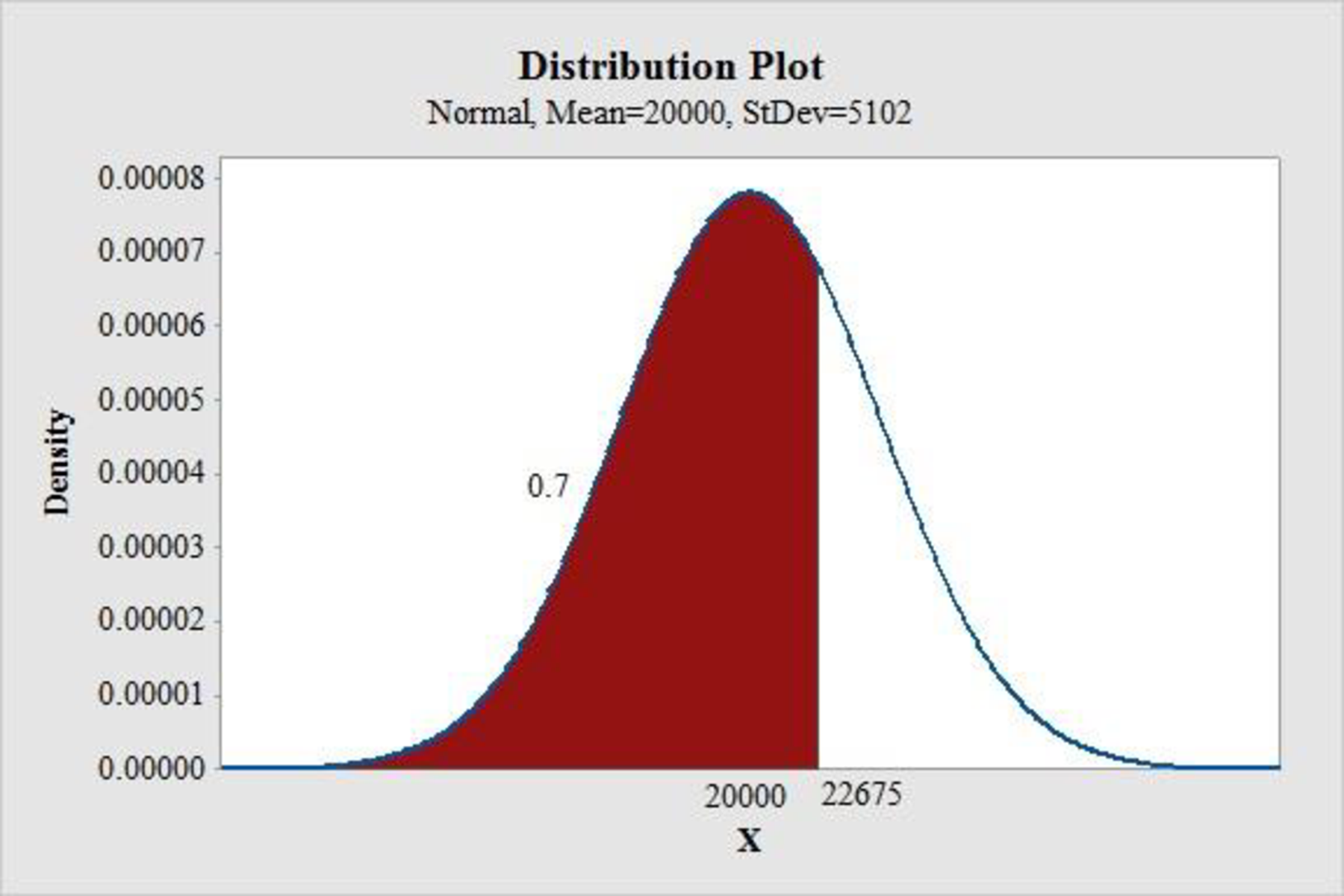
Thus, the quantity that would be ordered under the policy is 22,675.
The profit projections are obtained with the similar calculations made in part(c) for an order quantity of 22,675 units and is given in the following table:
| Unit sales | Total cost ($) | At $24 | At $5 | Profit($) |
| 10,000 | 362,800 | 240,000 | 63,375 | –59,425 |
| 20,000 | 362,800 | 480,000 | 13,375 | 130,575 |
| 30,000 | 362,800 | 544,200 | 0 | 181,400 |
5.
Provide the recommendation for an order quantity and note the associated profit projections and provide the rationale for the recommendation.
Explanation of Solution
A variety of recommendations are possible. From the three scenarios used in part (c) and (d) it is clear that an order quantity in the range 18,000 to 20,000 will be good to generate profit. Because the order quantities of more than 20,000 units generates a risk of loss and reduces the chance of generating good profits.
Want to see more full solutions like this?
Chapter 6 Solutions
EBK STATISTICS FOR BUSINESS & ECONOMICS


- The Vintage Restaurant, on Captiva Island near Fort Myers, Florida, is owned and operated by Karen Payne. The restaurant just completed its third year of operation. Since opening her restaurant, Karen has sought to establish a reputation for the Vintage as a high-quality dining establishment that specializes in fresh seafood. Through the efforts of Karen and her staff, her restaurant has become one of the best and fastest growing restaurants on the island. To better plan for future growth of the restaurant, Karen needs to develop a system that will enable her to forecast food and beverage sales by month for up to one year in advance. Table 17.25 shows the value of food and beverage sales ($1000s) for the first three years of operation. Dependent variable: What is the variable: ___________________________________________ How it is measured, i.e. what units or categories are used (e.g., revenue measured in “dollars”; height measured as “short, average, tall”)…arrow_forwardThe Vintage Restaurant, on Captiva Island near Fort Myers, Florida, is owned and operated by Karen Payne. The restaurant just completed its third year of operation. Since opening her restaurant, Karen has sought to establish a reputation for the Vintage as a high-quality dining establishment that specializes in fresh seafood. Through the efforts of Karen and her staff, her restaurant has become one of the best and fastest growing restaurants on the island. To better plan for future growth of the restaurant, Karen needs to develop a system that will enable her to forecast food and beverage sales by month for up to one year in advance. Table 17.25 shows the value of food and beverage sales ($1000s) for the first three years of operation. Managerial Report Perform an analysis of the sales data for the Vintage Restaurant. Prepare a report for Karen that summarizes your findings, forecasts, and recommendations. Include the following: A time series plot. Comment on the underlying pattern…arrow_forwardThe college graduates of 2000 could hardly have asked for better luck. The unemployment rate dropped to 4.1 % in May 2000- roughly, the lowest level in a generation- and employers were literally scrambling for new hires. Starting salaries rose, many graduating seniors had numerous job offers, and some firms even offered $10,000- $20,000 bonuses to students who signed the dotted line. Three years later, the job market for the Class of 2003 was rather different. U.S. economic growth had slowed to a crawl, and then to a halt. Companies that had stocked up on recent college grads in the tighter labour markets of 1998-2000 found themselves with more than they knew what to do with in 2002 and 2003. They were not eager to hire more. Bonuses and other “perks” disappeared; job offers became scarcer. With the unemployment rate around 6% in May and June of 2003, the job market was far from the worst ever. But it was nothing like the glory days of 2000. YOU ARE REQUIRED TO: (iv) Briefly…arrow_forward
- New legislation passed in 2017 by the U.S. Congress changed tax laws that affect how many people file their taxes in 2018 and beyond. These tax law changes will likely lead many people to seek tax advice from their accountants (The New York Times). Backen and Hayes LLC is an accounting firm in New York state. The accounting firm believes that it may have to hire additional accountants to assist with the increased demand in tax advice for the upcoming tax season. Backen and Hayes LLC has developed the following probability distribution for a = number of new clients seeking tax advice. Excel File: data05-19.xlsx f(x) 20 0.05 25 0.20 30 0.25 35 0.15 40 0.15 45 0.10 50 0.10 a. Is this a valid probability distribution? - Select your answer - Explain. f(z) Select your answer - - Select your answer b. What is the probability that Backen and Hayes LLC will obtain 40 or more new clients (to 2 decimals)? c. What is the probability that Backen and Hayes LLC will obtain fewer than 35 new clients…arrow_forwardThe Lawson Fabric Mill Produces five different fabrics. Each fabric can be woven on one or more of the mill’s 36 looms. The sales department’s forecast of demand for the next month is shown in below Table 1, along with data on the selling price per yard, variable cost per yard, and purchase price per yard. The mill operates 24 hours a day and is scheduled for 30 days during the coming month. The mill has two types of looms: draw and regular. The draw looms are more versatile and can be used for all five fabrics. The regular looms can produce only three of the fabrics. The mill has a total of 36 looms: 8 are draw and 28 are regular. The rate of production for each fabric on each type of loom is given in below Table 2. The time required to change over from producing one fabric to another is negligible and does not have to be considered. The Lawson Fabric Mill satisfies all demand with either its own fabric or fabric purchased from another mill. Fabrics that cannot be woven at the…arrow_forwardNew legislation passed in 2017 by the U.S. Congress changed tax laws that affect how many people file their taxes in 2018 and beyond. These tax law changes will likely lead many people to seek tax advice from their accountants (The New York Times). Backen and Hayes LLC is an accounting firm in New York state. The accounting firm believes that it may have to hire additional accountants to assist with the increased demand in tax advice for the upcoming tax season. Backen and Hayes LLC has developed the following probability distribution for number of new clients seeking tax advice. x f(x) 20 0.05 25 0.20 30 0.25 35 0.15 40 0.15 45 0.10 50 0.10 b. What is the probability that Backen and Hayes LLC will obtain 40 or more new clients (to 2 decimals c. What is the probability that Backen and Hayes LLC will obtain fewer than 35 new clients (to 2 decimals)? d.Compute the expected value, variance, and standard deviation of (to 2 decimals). Expected value…arrow_forward
- New legislation passed in 2017 by the U.S. Congress changed tax laws that affect how many people file their taxes in 2018 and beyond. These tax law changes will likely lead many people to seek tax advice from their accountants (The New York Times). Backen and Hayes LLC is an accounting firm in New York state. The accounting firm believes that it may have to hire additional accountants to assist with the increased demand in tax advice for the upcoming tax season. Backen and Hayes LLC has developed the following probability distribution for * = number of new clients seeking tax advice. Excel File: data05-19.xlsx f(2) 20 0.05 25 0.20 30 0.25 35 0.15 40 0.15 45 0.10 50 0.10 a. Is this a valid probability distribution? - Select your answer - Explain. f(x) Select your answer - Select your answer - b. What is the probability that Backen and Hayes LLC will obtain 40 or more new clients (to 2 decimals)? c. What is the probability that Backen and Hayes LLC will obtain fewer than 35 new clients…arrow_forwardThree businesswomen are trying to convene in Cincinnati for a business meeting. The first women (Woman 1) is arriving on a flight from Atlanta, the second (Woman 2) is arriving on a flight from Dallas, and the third (Woman 3) is arriving on a flight from Chicago. Historical data suggests that the Atlanta flight is “on time” 90% of the time, the Dallas flight is “on time” 95% of the time, and the Chicago flight is “on time” 80% of the time. Furthermore, historical data suggests that the three flights are independent with respect to on time behavior. Define the sample space for this random experiment. Compute the probability for each of the outcomes in the sample space. Let W denote the number of business women that arrive on time. Construct the probability mass function of W Construct the cumulative distribution function of W Find the expected value of W Compute the standard deviation of Warrow_forwardEvery month a clothing store conducts an inventory and calculates losses from theft. The store would like to reduce these losses and is considering two methods. The first is to hire a security guard, and the second is to install cameras. To help decide which method to choose, the manager hired a security guard for 6 months. During the next 6-month period, the store installed cameras. The monthly losses were recorded and are listed here. The manager decided that because the cameras were cheaper than the guard, he would install the cameras unless there was enough evidence to infer that the guard was better. What should the manager do? Security guard Cameras 355 284 401 398 477 254 486 303 270 386 411 435arrow_forward
- A loan officer knows that 50% of loan applicants in their 20s have bad credit, 40% of loan applicants in their 30s have bad credit, and 20% of loan applicants age 40 or greater have bad credit. She also knows that 30% of loan applicants are in their 20s, 50% are in their 30s, and the rest are at least 40 years of age. What percentage of applicants with bad credit are at least 40 years old? Explain the steps you took to determine answer.arrow_forwardThe Ashland MultiComm Services (AMS) marketing department wants to increase subscriptions for its 3-For-All telephone, cable, and Internet combined service. To ensure that as many trial subscriptions to the 3-For-All service as possible are converted to regular subscriptions, the marketing department works closely with the customer support department to accomplish a smooth initial process for the trial subscription customers. To assist in this effort, the marketing department needs to accurately forecast the monthly total of new regular subscriptions. A team consisting of managers from the marketing and customer support departments was convened to develop a better method of forecasting new subscriptions. Previously, after examining new subscription data for the prior three months, a group of three managers would develop a subjective forecast of the number of new subscriptions. Livia Salvador, who was recently hired by the company to provide expertise in quantitative forecasting…arrow_forwardA salon owner estimates the number of clients she is expecting during the festive season to be 20% during Monday to Wednesday, 20% on Thursday and 60% over the weekend. She therefore hires additional staff to assist during the weekend to meet the client demand. She however only observes 30% during Monday to Wednesday, 20% on Thursday and 50% over the weekend in the first week of December. The salon owner is uncertain whether she should reduce the planned staff for the December festive period due the observed trend or not. She conducts a statistical test at α = 0.05 to determine if the observed trend fits the expected trend. Which of the following statements is true? A. The conclusion of the test is that she should not keep the additional staff for the weekend. B. The df for this test is 3. C. The p-value is greater than α. D. The null hypothesis is that the observed trend is different to the expected trend. E. The test statistic is χ2 = 5.33.arrow_forward
 MATLAB: An Introduction with ApplicationsStatisticsISBN:9781119256830Author:Amos GilatPublisher:John Wiley & Sons Inc
 Probability and Statistics for Engineering and th...StatisticsISBN:9781305251809Author:Jay L. DevorePublisher:Cengage Learning
 Statistics for The Behavioral Sciences (MindTap C...StatisticsISBN:9781305504912Author:Frederick J Gravetter, Larry B. WallnauPublisher:Cengage Learning
 Elementary Statistics: Picturing the World (7th E...StatisticsISBN:9780134683416Author:Ron Larson, Betsy FarberPublisher:PEARSON
 The Basic Practice of StatisticsStatisticsISBN:9781319042578Author:David S. Moore, William I. Notz, Michael A. FlignerPublisher:W. H. Freeman
 Introduction to the Practice of StatisticsStatisticsISBN:9781319013387Author:David S. Moore, George P. McCabe, Bruce A. CraigPublisher:W. H. Freeman