
CONTROL SYSTEMS ENGINEERING
7th Edition
ISBN: 9781119185666
Author: NISE
Publisher: WILEY
expand_more
expand_more
format_list_bulleted
Concept explainers
Videos
Textbook Question
Chapter 7, Problem 2P
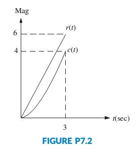
Figure P7.2 shows the ramp input r(t) and the output c(t) of a system. Assuming the output’s steady state can be approximated by a ramp, find [Section: 7.1]
a. the steady-state error;
b. the steady-state error if the input becomes r(t) =tu(t).
Expert Solution & Answer
Want to see the full answer?
Check out a sample textbook solution
Students have asked these similar questions
Feedback & Control Systems
State-Space Representation
Write the state-space representation of the system
below. Let the output of the mechanical system is
x3 (t).
1 N-s/m
x₁ (t) M3 = 1kg
1 N/m
М1
-0000 1kg
> X3 (t)
1 N-s/m
1 N/m
oooo
x₂ (t)
M₂
1kg
4
1 N-s/m²
-1 N-s/m
→f(t)
Represent the translational mechanical system shown below in state space,
where x3(t) is the output.
State variables
ニュ=X
3 = X2
Let
-4 = X2
Es = X3
E6 = X3
x1(t)
x2(t)
x3(t)
1 N-sim
1 N-sim
1 Nim
1 Nim
1kg
1kg
1 kg
J1
J2
J3
Fit)
Consider the following mechanical system:
k
m
+f
b
d²y(t)
+b-
dy(t)
+ ky(t) = f (t)
m
%3D
dt?
dt
Obtain the state space model of the system with input f (t) and output y(t). Calculate
the system matrices for m = 1, k = 1 and b = 2.
Check the stability by using the second method of Lyapunov.
3.
Chapter 7 Solutions
CONTROL SYSTEMS ENGINEERING
Ch. 7 - Prob. 1RQCh. 7 - A position control, tracking with a constant...Ch. 7 - Name the test inputs used to evaluate steady-state...Ch. 7 - Prob. 4RQCh. 7 - Increasing system gain has what effect upon the...Ch. 7 - Prob. 6RQCh. 7 - Prob. 7RQCh. 7 - Prob. 8RQCh. 7 - Prob. 9RQCh. 7 - The forward transfer function of a control system...
Ch. 7 - Prob. 11RQCh. 7 - Prob. 12RQCh. 7 - Is the forward-path actuating signal the system...Ch. 7 - Prob. 14RQCh. 7 - Prob. 15RQCh. 7 - Name two methods for calculating the steady-state...Ch. 7 - Prob. 1PCh. 7 - Figure P7.2 shows the ramp input r(t) and the...Ch. 7 - Prob. 3PCh. 7 - Prob. 4PCh. 7 - Prob. 5PCh. 7 - Prob. 6PCh. 7 - Prob. 7PCh. 7 - Prob. 8PCh. 7 - A system has Kp = 4. What steady-state error can...Ch. 7 - Prob. 10PCh. 7 - Prob. 11PCh. 7 - Prob. 12PCh. 7 - For the system shown in Figure P7.4. [Section:...Ch. 7 - Prob. 14PCh. 7 - 1515. Find the system type for the system of...Ch. 7 - Prob. 16PCh. 7 - Prob. 17PCh. 7 - Prob. 18PCh. 7 - Prob. 19PCh. 7 - Given the system of Figure P7.8, design the value...Ch. 7 - Prob. 21PCh. 7 - Prob. 22PCh. 7 - Prob. 23PCh. 7 - Prob. 24PCh. 7 - Prob. 25PCh. 7 - Prob. 26PCh. 7 - Prob. 27PCh. 7 - Prob. 28PCh. 7 - Prob. 29PCh. 7 - Prob. 30PCh. 7 - Prob. 31PCh. 7 - Prob. 32PCh. 7 - Given the system in Figure P7.9, find the...Ch. 7 - Repeat Problem 33 for the system shown in Figure...Ch. 7 - Prob. 36PCh. 7 - Prob. 37PCh. 7 - Prob. 38PCh. 7 - Design the values of K1and K2in the system of...Ch. 7 - Prob. 41PCh. 7 - For each system shown in Figure P7.17, find the...Ch. 7 - For each system shown in Figure P7.18, find the...Ch. 7 - Prob. 44PCh. 7 - 45. For the system shown in Figure P7.20,...Ch. 7 - Prob. 47PCh. 7 - Prob. 48PCh. 7 - Prob. 49PCh. 7 - Prob. 50PCh. 7 - Prob. 51PCh. 7 - Prob. 52PCh. 7 - Prob. 53PCh. 7 - Prob. 54PCh. 7 - Prob. 55PCh. 7 - Prob. 58PCh. 7 - Prob. 59PCh. 7 - Prob. 62PCh. 7 - Prob. 63PCh. 7 - Prob. 64PCh. 7 - Prob. 65PCh. 7 - Prob. 66PCh. 7 - Prob. 67PCh. 7 - Prob. 68P
Knowledge Booster


Learn more about
Need a deep-dive on the concept behind this application? Look no further. Learn more about this topic, mechanical-engineering and related others by exploring similar questions and additional content below.Similar questions
- Given a state space model [1 1 + 0 u -1 -2 y = [1 1 0] with input u and output y. a). Derive the transfer function representation. b). Derive the differential equations representation. c). Compute the response y(t) with step control input u(t) = 1(t) and zero initial condition. d). and initial condition r(0) = [11 0]". Compute the state response r(t) with control input u(t) = 1(t)arrow_forward11. Consider a system that can be modeled as shown. The input x in (t) is a prescribed motion at the right end of spring k 2. Find X(s) the system transfer function Xeq(s)* m k₂ ww Xin The values of the parameters are m= 30 kg, k ₁=700 N/m, k 2= 1300 N/m, and b=200 N- s/m. Write a MATLAB script file that: (a) calculates the natural frequency, damping ratio, and damped natural frequency for the system; and (b) uses the impulse command to find and plot the response of the system to a unit impulse input.arrow_forwardUse MATLAB to obtain a state model for the following equations; obtain the expressions for the matrices A, B, C, and D. In both cases, the input is f(t); the output: is y. a. 5d³yd²y +7. b. dy +3 dt³ dt² dt Y(s) 5 = F(s) s² +7s+4 - +6y=f(t)arrow_forward
- B₁ 1*1* X1 A x2 (a) Identify state variables. (b) Find the state equations. K www M XXXX fa(t) B₂ For the system shown in the figure above, differential model equations are given below. B₁x₁ + Kx₁Kx₂ = 0 MX₂ + B₂x₂ + Kx₂ - Kx₁ = fa(t)arrow_forwardLook at the block diagram for the dynamic model of the hydraulically actuated system in Fig where: km = 0.2 J = 0.1 m = 5 k₂ = 3 L₂ = 2 KAP = 4 *BÖH Lu da K₁ W *ÖDDÖDDÖD D Km/J X4 QmJ/Km K₁pJ 1. Determine the controllability and observability for this system d₂ X3 X₂ Aarrow_forward2. Consider the state equation x1 1 20 x1 d x2 = 0 10 x2 dt x3 001 x3 where x1, x2 and 23 are state variables. Please answer the following questions. (a) The state matrix (4) 1 20 A = 0 1 0 (5) 0 0 1 has three-fold eigenvalues with \₁ = = A2 A3 1. Find all independent eigenvectors corresponding to this eigenvalue. (b) Find the modal matrix M associated with the state matrix A. Does M-1 AM lead to a Jordan form or not? Hint: The modal matrix M turns out to be a diagonal matrix. For a diagonal matrix, its inverse is given by a 00 0b0 -1 1/a 0 0 = 0 1/b 0 00 с 0 0 1/c 1 (6) (c) Find the state transition matrix (t). (d) Determine the stability of the system. Please justify your answer.arrow_forward
- #3) a) Show that the below given system has the following representation where u=x. 1 cl %3D b) Plot the impulse response of the system for m=10, c=3, k=5,1,=l½/2=l3/2=1. c) Find the transfer functions, poles and zeros of the system. #4) a) Show that the state space respresentation of the cartesian elbow manipulator is as given below. b) Assuming unit values for all constants, plot the q, and q, angles for 5 seconds for the nonzero initial conditions (q,lo= (q;)o=30°. c) Find the transfer functions, poles and zeros of the system.arrow_forwardasaparrow_forward1%9• l1, ie O 10:YE Consider the system presented by the following transfer function y(s) s+2 и (s) + 2s +3 The state-space model is A = -2 C=[2 1] D=[2] а. B = b. A= B = |-3 -2 C=[1 0] D=[0] c. A = B = -3 d. A= C =[2 1] D=[0] B = -3 -2 Select one: O a. d O b. a II > IIarrow_forward
- Q4) A particular control system yielded a steady state error of 0.20 for unit step input. A unit integrator is cascaded to this system and unit ramp input is applied to this modified system. What is the value of steady-state error for this modified system?arrow_forwardFor the following state-space representation,define the:– State Vector– System Matrix– Feedforward Matrix– Input Matrix & Input Vector– Output Matrix & Output Vectorarrow_forward2- Using Matlab, what are the step response curves of the closed-loop system, as shown in fig.1. the feedback represents the second-order dynamic system. (fill in the following table) For=0.4 Wn 1 3 6 9 10 R(S) 0.1 0.3 0.6 0.9 1 For w 5 rad/sec 3 Settling time Peak response 2 Wn s(s+23wn) Settling time Peak response C(s) Discuss the follow Which parameters or w occur on the rise time of the response? Which parameter increases the speed of response? Which parameters can be decreases the response amplitude? Which parameter decreases the steady error state? fig.2arrow_forward
arrow_back_ios
SEE MORE QUESTIONS
arrow_forward_ios
Recommended textbooks for you
 Elements Of ElectromagneticsMechanical EngineeringISBN:9780190698614Author:Sadiku, Matthew N. O.Publisher:Oxford University Press
 Mechanics of Materials (10th Edition)Mechanical EngineeringISBN:9780134319650Author:Russell C. HibbelerPublisher:PEARSON
 Thermodynamics: An Engineering ApproachMechanical EngineeringISBN:9781259822674Author:Yunus A. Cengel Dr., Michael A. BolesPublisher:McGraw-Hill Education
 Control Systems EngineeringMechanical EngineeringISBN:9781118170519Author:Norman S. NisePublisher:WILEY
 Mechanics of Materials (MindTap Course List)Mechanical EngineeringISBN:9781337093347Author:Barry J. Goodno, James M. GerePublisher:Cengage Learning
 Engineering Mechanics: StaticsMechanical EngineeringISBN:9781118807330Author:James L. Meriam, L. G. Kraige, J. N. BoltonPublisher:WILEY
Elements Of Electromagnetics
Mechanical Engineering
ISBN:9780190698614
Author:Sadiku, Matthew N. O.
Publisher:Oxford University Press
Mechanics of Materials (10th Edition)
Mechanical Engineering
ISBN:9780134319650
Author:Russell C. Hibbeler
Publisher:PEARSON
Thermodynamics: An Engineering Approach
Mechanical Engineering
ISBN:9781259822674
Author:Yunus A. Cengel Dr., Michael A. Boles
Publisher:McGraw-Hill Education
Control Systems Engineering
Mechanical Engineering
ISBN:9781118170519
Author:Norman S. Nise
Publisher:WILEY
Mechanics of Materials (MindTap Course List)
Mechanical Engineering
ISBN:9781337093347
Author:Barry J. Goodno, James M. Gere
Publisher:Cengage Learning
Engineering Mechanics: Statics
Mechanical Engineering
ISBN:9781118807330
Author:James L. Meriam, L. G. Kraige, J. N. Bolton
Publisher:WILEY
Ch 2 - 2.2.2 Forced Undamped Oscillation; Author: Benjamin Drew;https://www.youtube.com/watch?v=6Tb7Rx-bCWE;License: Standard youtube license