
a.
To construct: The
a.
Answer to Problem 7.40TY
Output using the MINITAB software is given below:
Explanation of Solution
Given info:
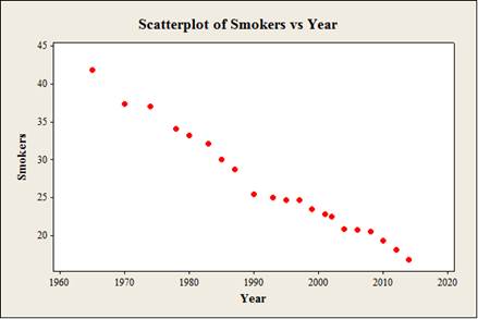
The data shows the year (x) and smokers (y) values.
Calculation:
Step by step procedure to obtain scatterplot using the MINITAB software:
- Choose Graph > Scatterplot.
- Choose Simple and then click OK.
- Under Y variables, enter a column of Smokers.
- Under X variables, enter a column of Year.
- Click OK.
Observation:
From the plot, it is observed that the horizontal axis represents year and vertical axis represents smokers.
b.
To describe: The direction, form, and strength of the relationship between the year and smokers.
To identify: Whether there are any outliers.
b.
Answer to Problem 7.40TY
There is negative direction from the overall pattern.
There is linear form from the overall pattern.
There is a strong relationship between the year and smokers.
There are no outliers from the overall pattern.
Explanation of Solution
Here, the scatterplot is used to describe the direction, form, and strength of the relationship between the year and smokers. Also, the scatterplot is used for identifying the outliers from the overall pattern.
Direction:
The direction shows the overall pattern of the variables. That is, whether the points move from lower left to upper right or from upper left to lower right.
From the scatterplot, it is observed that there is negative direction between the year and smokers because the data points are scattered and move from upper left to lower right.
Form:
The form gives the information about whether the points closely form a straight line, curved or oscillate in some way. That is, it explains about the
From the scatterplot, it is observed that there is linear form between the year and smokers because the data points show the distinct pattern.
Strength:
The strength tells about the overall relationship, that is, whether it is a strong relationship or weak relationship.
Here, from the scatterplot, it is observed that there is a strong relationship between the year and smokers because the data points are closely scattered.
Hence, the relationship was very strong.
Justification:
Outlier:
An observation is said to be an outlier if it is far away from the other observations.
From the scatterplot, it is observed that there is no value which is far away from the other observations. Thus, there is no outlier in the overall pattern.
c.
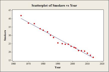
To find: The equation of the least-squares regression line with year (x) as the predictor variable.
To construct: The scatterplot with regression line for the variables year and smokers.
c.
Answer to Problem 7.40TY
The equation of the least-squares regression line with year as the predictor variable (x) is
Output using the MINITAB software is given below:
Explanation of Solution
Calculation:
Regression:
Software procedure:
Step by step procedure to find the equation of the least-squares line by using the MINITAB software:
- Choose Stat > Regression > Regression.
- In Responses, enter the column of Smokers.
- In Predictors, enter the column of Year.
- Click OK.
Output using the MINITAB software is given below:
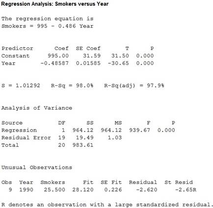
From the MINITAB output, the equation of the least-squares regression line for smokers with year is
Scatterplot:
Step by step procedure to construct the scatterplot using the MINITAB software:
- Choose Graph > Scatterplot.
- Choose With Regression, and then click OK.
- In Responses, enter the column of Smokers.
- In Predictors, enter the column of Year.
- Click OK.
d.
To obtain: Average decrease in smoking per year from 1965 to 2014.
d.
Answer to Problem 7.40TY
The average decrease in smoking per year from 1965 to 2014 is –0.486.
Explanation of Solution
Slope:
It is states the predicted value of y for any given value of x since the response variable (y) is dependent on explanatory variable (x).
Here, the coefficient of x is –0.486. Hence, the slope of the line is negative.
The interpretation for the slope of the line is that, the coefficient value for x is –0.486. Also, the slope indicates for increase in each year, the smokers are decreased by
Thus, the average decrease in smoking per year from 1965 to 2014 is –0.486.
e.
To obtain: The percentage of the observed variation in percent of adults who smoke can be explained by linear change over time.
e.
Answer to Problem 7.40TY
The percentage of the observed variation in percent of adults who smoke can be explained by linear change over time is 98%.
Explanation of Solution
From the MINITAB output for regression in part (c), it is observed that the
Also, the
f.
To find: The predicted the percent of adults who will smoke in 2020.
f.
Answer to Problem 7.40TY
The predicted the percent of adults who will smoke in 2020 is 13.28.
Explanation of Solution
Calculation:
The predicted the percent of adults who will smoke in 2020 is,
Thus, the predicted the percent of adults who will smoke in 2020 is 13.28.
g.
To find: The predicted the percent of adults who will smoke in 2075.
To explain: The reason that the result is impossible.
To explain: The reason that the prediction is made by the regression line to be foolish.
g.
Answer to Problem 7.40TY
The predicted the percent of adults who will smoke in 2075 is –13.45.
The prediction value is impossible because the predicted value of smokers is negative.
The prediction is made by the regression line is foolishness because year 2075 leads to extrapolation.
Explanation of Solution
Calculation:
The predicted the percent of adults who will smoke in 2075 is,
Thus, the predicted the percent of adults who will smoke in 2075 is –13.45. So, the predicted value of smokers is negative.
Hence, the prediction value is impossible.
Justification:
The period of time is from 2014 to 2045. Thus, the year 2075 is far beyond the
Want to see more full solutions like this?
Chapter 7 Solutions
BASIC PRACTICE OF STATISTICS >C<

 MATLAB: An Introduction with ApplicationsStatisticsISBN:9781119256830Author:Amos GilatPublisher:John Wiley & Sons Inc
 Probability and Statistics for Engineering and th...StatisticsISBN:9781305251809Author:Jay L. DevorePublisher:Cengage Learning
 Statistics for The Behavioral Sciences (MindTap C...StatisticsISBN:9781305504912Author:Frederick J Gravetter, Larry B. WallnauPublisher:Cengage Learning
 Elementary Statistics: Picturing the World (7th E...StatisticsISBN:9780134683416Author:Ron Larson, Betsy FarberPublisher:PEARSON
 The Basic Practice of StatisticsStatisticsISBN:9781319042578Author:David S. Moore, William I. Notz, Michael A. FlignerPublisher:W. H. Freeman
 Introduction to the Practice of StatisticsStatisticsISBN:9781319013387Author:David S. Moore, George P. McCabe, Bruce A. CraigPublisher:W. H. Freeman