Videos
a.
Verify that
a.
Explanation of Solution
Step-by-step procedure to obtain the average using Ti-83 calculator:
- Click on Stat.
- From EDIT, choose 1: Edit..
- In column L1, enter the data.
- Click on Stat.
- From CALC, choose 1: 1-Var Stats.
- Select 2nd > 1.
- Click Enter.
Output obtained is as follows:
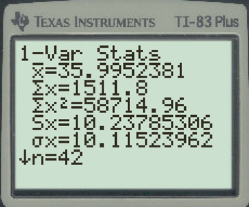
From the output, the value of average is obtained as 35.9952
It is verified that
b.
Obtain the 75% confidence interval for
b.
Answer to Problem 23P
The 75% confidence interval for
Explanation of Solution
Here,
From Table 5: Areas of a Standard
The 75% confidence interval for
Therefore, the 75% confidence interval for
c.
Explain whether the annual profit of less than 30 thousand dollars is low when compared with other successful financial institutions.
c.
Explanation of Solution
From Part (b), the 75% confidence interval for
Since all the values in the interval are greater than 30, it is clear that the annual profit of less than 30 thousand dollars is low when compared with other successful financial institutions.
d.
Explain whether the annual profit of more than 40 thousand dollars is better when compared with other successful financial institutions.
d.
Explanation of Solution
From Part (b), the 75% confidence interval for
Here, all the values in the interval are less than 40. That is, 40 thousand dollars is greater than the upper bound of the interval. Therefore, the annual profit of more than 40 thousand dollars is better when compared with other successful financial institutions.
e.
Find the 90% confidence interval for
e.
Answer to Problem 23P
The 90% confidence interval for
The 90% confidence interval for
Explanation of Solution
Here,
From Table 5: Areas of a Standard Normal Distribution, the value corresponding to 0.0495 (which is approximately 0.05) is –1.65. That is,
The 90% confidence interval for
Therefore, the 90% confidence interval for
The 90% confidence interval for
Therefore, the 90% confidence interval for
Want to see more full solutions like this?
Chapter 7 Solutions
Understandable Statistics: Concepts and Methods


- Urban Travel Times Population of cities and driving times are related, as shown in the accompanying table, which shows the 1960 population N, in thousands, for several cities, together with the average time T, in minutes, sent by residents driving to work. City Population N Driving time T Los Angeles 6489 16.8 Pittsburgh 1804 12.6 Washington 1808 14.3 Hutchinson 38 6.1 Nashville 347 10.8 Tallahassee 48 7.3 An analysis of these data, along with data from 17 other cities in the United States and Canada, led to a power model of average driving time as a function of population. a Construct a power model of driving time in minutes as a function of population measured in thousands b Is average driving time in Pittsburgh more or less than would be expected from its population? c If you wish to move to a smaller city to reduce your average driving time to work by 25, how much smaller should the city be?arrow_forwardRunning Speed A man is running around a circular track that is 200 m in circumference. An observer uses a stopwatch to record the runner’s time at the each of each lap, obtaining the data in the following table. (a) What was the man’s average speed (rate) between 68 s and 152 s? (b) What was the man’s average speed between 263 s and 412 s? (c) Calculate the man’s speed for cadi lap, Is he slowing down, speeding up, or neither?arrow_forward
 Functions and Change: A Modeling Approach to Coll...AlgebraISBN:9781337111348Author:Bruce Crauder, Benny Evans, Alan NoellPublisher:Cengage Learning
 Algebra & Trigonometry with Analytic GeometryAlgebraISBN:9781133382119Author:SwokowskiPublisher:Cengage
 Linear Algebra: A Modern IntroductionAlgebraISBN:9781285463247Author:David PoolePublisher:Cengage Learning
 College AlgebraAlgebraISBN:9781305115545Author:James Stewart, Lothar Redlin, Saleem WatsonPublisher:Cengage Learning