Chapter 7.4, Problem 9E

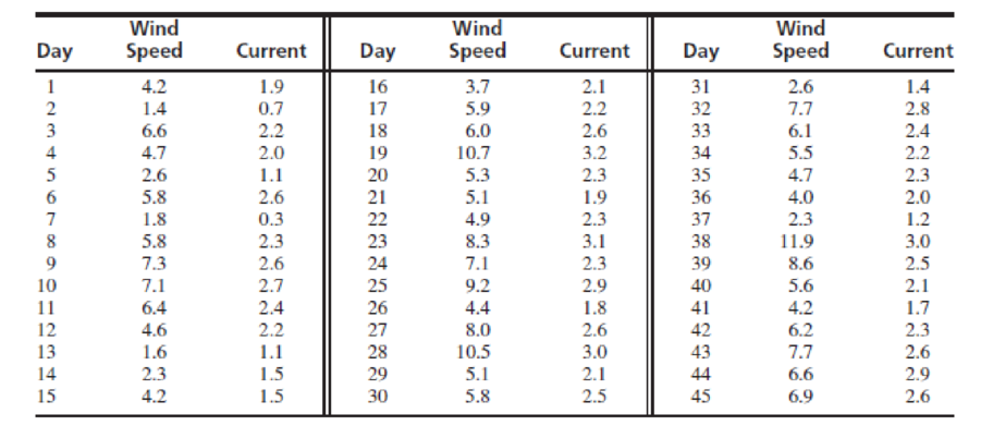
A windmill is used to generate direct current. Data are collected on 45 different days to determine the relationship between wind speed in mi/h (x) and current in kA (y). The data are presented in the following table.

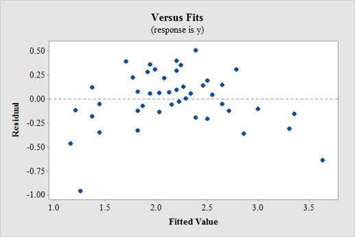
1. a. Compute the least-squares line for predicting y from x. Make a plot of residuals versus fitted values.
2. b. Compute the least-squares line for predicting y from ln x. Make a plot of residuals versus fitted values.
3. c. Compute the least-squares line for predicting ln y from x. Make a plot of residuals versus tilted values.
4. d. Compute the least-squares line for predicting $\sqrt{y}$ from x. Make a plot of residuals versus fitted values.
5. e. Which of the four models (a) through (d) fits best? Explain.
6. f. For the model that fits best, plot the residuals versus the order in which the observations were made. Do the residuals seem to vary with time?
7. g. Using the best model, predict the current when wind speed is 5.0 mi/h.
8. h. Using the best model, find a 95% prediction interval for the current on a given day when the wind speed is 5.0 mi/h.

To determine

Compute the least-squares line for predicting y from x and plot the residuals versus the fitted values.

Answer to Problem 9E

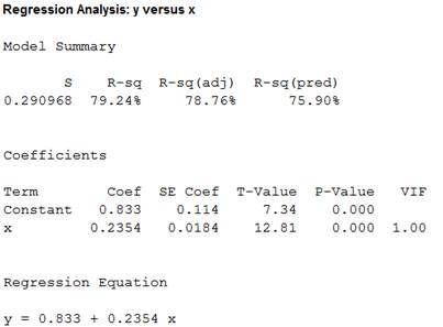
The least-squares line for predicting y from x is $y=0.833+ 0.2354 x$.

Explanation of Solution

Given info:

The data represents the wind speed in mi/h (x) and current in kA (y) for 45 different days.

Calculation:

Software Procedure:

Step-by-step procedure to obtain the least-squares line and also construct the residuals versus the fitted plot using the MINITAB software is given below:

• Choose Stat > Regression > Regression > Fit Regression Model.
• In Responses, enter “y”.
• In Continuous predictors, enter “x”.
• Check Results.
• In Graph, choose residual versus fits.
• In Display of results, choose Simple tables.
• Click OK.

Output using the MINITAB software is given below:

Residual versus fits:

From the MINITAB output, the least-squares line for predicting y from x is $y=0.833+ 0.2354 x$.

To determine

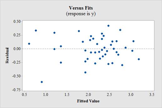
Compute the least-squares line for predicting y from ln x and plot the residuals versus the fitted values.

Answer to Problem 9E

The least-squares line for predicting y from ln x is $y=0.199+ 1.2066 \ln x$.

Explanation of Solution

Calculation:

Software Procedure:

Step-by-step procedure to obtain the least-squares line and also construct the residuals versus the fitted plot using the MINITAB software is given below:

• Choose Stat > Regression > Regression > Fit Regression Model.
• In Responses, enter “y”.
• In Continuous predictors, enter “ln x”.
• Check Results.
• In Graph, choose residual versus fits.
• In Display of results, choose Simple tables.
• Click OK.

Output using the MINITAB software is given below:

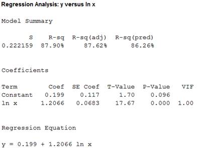
Residual versus fits:

From the MINITAB output, the least-squares line for predicting y from ln x is $y=0.199+ 1.2066 \ln x$.

To determine

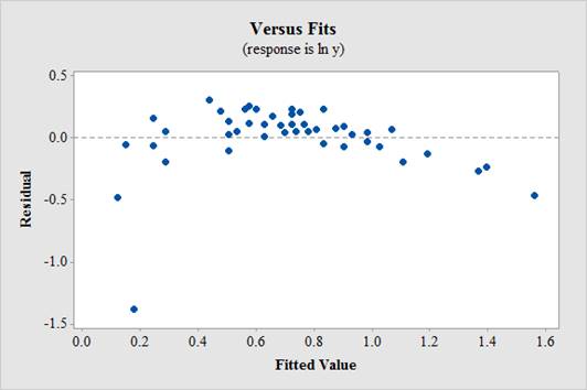
Compute the least-squares line for predicting ln y from x and plot the residuals versus the fitted values.

Answer to Problem 9E

The least-squares line for predicting ln y from x is $\ln y=-0.068+ 0.1367 x$.

Explanation of Solution

Calculation:

Software Procedure:

Step-by-step procedure to obtain the least-squares line and also construct the residuals versus the fitted plot using the MINITAB software is given below:

• Choose Stat > Regression > Regression > Fit Regression Model.
• In Responses, enter “ln y”.
• In Continuous predictors, enter “x”.
• Check Results.
• In Graph, choose residual versus fits.
• In Display of results, choose Simple tables.
• Click OK.

Output using the MINITAB software is given below:

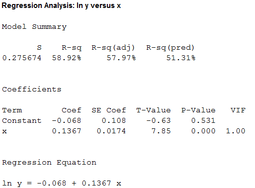
Residual versus fits:

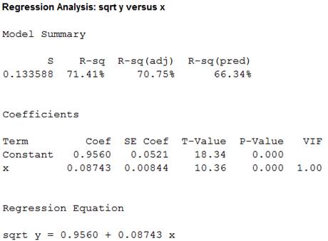
From the MINITAB output, the least-squares line for predicting ln y from x is $\ln y=-0.068+ 0.1367 x$.

To determine

Compute the least-squares line for predicting $\sqrt{y}$ from x and plot the residuals versus the fitted values.

Answer to Problem 9E

The least-squares line for predicting $\sqrt{y}$ from x is $\sqrt{y}\text{ = 0}\text{.9560 + 0}\text{.08743} x$.

Explanation of Solution

Calculation:

Software Procedure:

Step-by-step procedure to obtain the least-squares line and also construct the residuals versus the fitted plot using the MINITAB software is given below:

• Choose Stat > Regression > Regression > Fit Regression Model.
• In Responses, enter “$\sqrt{y}$”.
• In Continuous predictors, enter “x”.
• Check Results.
• In Graph, choose residual versus fits.
• In Display of results, choose Simple tables.
• Click OK.

Output using the MINITAB software is given below:

Residual versus fits:

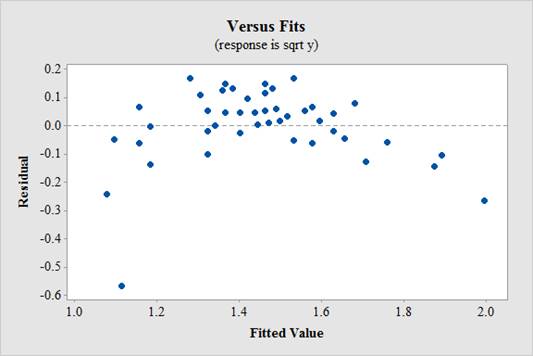
From the MINITAB output, the least-squares line for predicting $\sqrt{y}$ from x is $\sqrt{y}\text{ = 0}\text{.9560 + 0}\text{.08743} x$.

To determine

Identify the best fit of the model.

Answer to Problem 9E

The best fit of the model is $y=0.199+ 1.2066 \ln x$.

Explanation of Solution

Calculation:

From the above results, it can be observed the model $y=0.199+ 1.2066 \ln x$ is the best fit when compared to other models because the residual versus fitted plot shows the least pattern.

To determine

Plot the residuals versus order.

Explanation of Solution

Calculation:

Software Procedure:

Step-by-step procedure to construct the residuals versus order using the MINITAB software is given below:

• Choose Stat > Regression > Regression > Fit Regression Model.
• In Responses, enter “y”.
• In Continuous predictors, enter “ln x”.
• Check Results.
• In Graph, choose residual versus order.
• In Display of results, choose Simple tables.
• Click OK.

Output using the MINITAB software is given below:

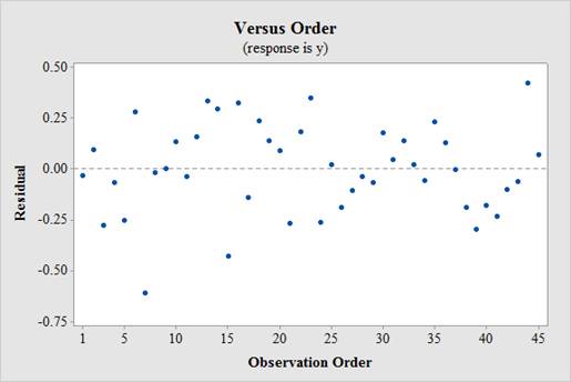
From the plot, it can be observed that the residual plot do not shows any pattern with time.

To determine

Predict the current when wind speed is 5.0 mi/h.

Answer to Problem 9E

The predicted value for current when wind speed is 5.0 mi/h is 2.14.

Explanation of Solution

Calculation:

Predicted value:

Software Procedure:

Step-by-step procedure to obtain the predicted value using the MINITAB software:

• Stat > Regression > Regression > Predict.
• In Responses, enter “y”.
• Choose Enter individual values.
• In “ln x”, enter 1.6094.
• Click OK.

Output using the MINITAB software is given below:

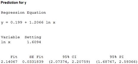
Thus, the predicted value for current when wind speed is 5.0 mi/h is 2.14.

To determine

Construct the 95% prediction interval for the current on a given day when the wind speed is 5.0 mi/h.

Answer to Problem 9E

The 95% prediction interval for the current on a given day when the wind speed is 5.0 mi/h is (1.68767, 2.59366).

Explanation of Solution

Calculation:

Prediction interval:

Software Procedure:

Step-by-step procedure to obtain the prediction interval using the MINITAB software:

• Stat > Regression > Regression > Predict.
• In Responses, enter “y”.
• Choose Enter individual values.
• In “ln x”, enter 1.6094.
• Click OK.

Output using the MINITAB software is given below:

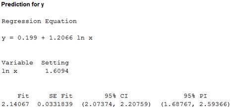
From the MINITAB output, the 95% prediction interval for the current on a given day when the wind speed is 5.0 mi/h is (1.68767, 2.59366).