
Subpart (a):
Calculate different costs.
Subpart (a):
Explanation of Solution
Total cost (TC) can be obtained by using the following formula.
Total cost at production level 1 unit can be calculated by substituting the respective values in Equation (1).
Total cost is $105.
Average fixed cost (AFC) can be obtained by using the following formula.
Average fixed cost at production level 1 unit can be calculated by substituting the respective values in Equation (2).
Average fixed cost is $60.
Average variable cost at production level 1 unit can be calculated by substituting the respective values in Equation (3).
Average variable cost is $45.
Total average cost at production level 1 unit can be calculated by substituting the respective values in Equation (4).
Average variable cost is $105.
Marginal cost (MC) can be obtained by using the following formula.
Average variable cost at production level 1 unit can be calculated by substituting the respective values in Equation (5).
Marginal cost is $105.
Table-1 shows the total cost, average fixed cost, average variable cost, average total cost and marginal cost that obtained by using equations (1), (2), (3), (4) and (5).
Table -1
| Quantity | Fixed cost | Variable cost | TC | AFC | AVC | AC | MC |
| 0 | 60 | 0 | 60 | ||||
| 1 | 60 | 45 | 105 | 60 | 45.00 | 105.00 | 45 |
| 2 | 60 | 85 | 145 | 30 | 42.50 | 72.50 | 40 |
| 3 | 60 | 120 | 180 | 20 | 40.00 | 60.00 | 35 |
| 4 | 60 | 150 | 210 | 15 | 37.50 | 52.50 | 30 |
| 5 | 60 | 185 | 245 | 12 | 37.00 | 49.00 | 35 |
| 6 | 60 | 225 | 285 | 10 | 37.50 | 47.50 | 40 |
| 7 | 60 | 270 | 330 | 8.57 | 38.57 | 47.14 | 45 |
| 8 | 60 | 325 | 385 | 7.50 | 40.63 | 48.13 | 55 |
| 9 | 60 | 390 | 450 | 6.67 | 43.33 | 50.00 | 65 |
| 10 | 60 | 465 | 525 | 6 | 46.50 | 52.50 | 75 |
Figure -1 illustrates the shape of total fixed cost, total cost and total variable cost that influencing by the diminishing returns to scale.
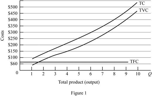
In figure -1, horizontal axis measures total output and vertical axis measures cost. The curve TC indicates total cost and the curve TVC indicates total variable cost. TFC curve indicates total fixed cost. Since total fixed cost is remain the same over the different level of production TFC curve parallel to the horizontal axis.
From the output range 1 unit to 4 units, total cost and total variable cost increasing at decreasing rate due to the increasing marginal returns. Thereafter, these two cost curves are increasing at increasing rate due to the diminishing marginal cost.
Concept introduction:
Fixed cost: Fixed costs refer to those costs that remain the same regardless of the level of production.
Variable cost: Variable cost refers to the costs that change due to the changes occurring in the level of production.
Subpart (b):
Calculate different costs.
Subpart (b):
Explanation of Solution
Figure -2 illustrates relationship between marginal cost, average variable cost, average fixed cost and average total cost curve.
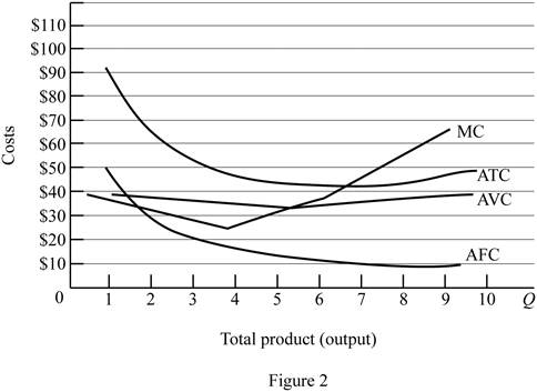
In figure -2, horizontal axis measures total output and vertical axis measures cost. The curve TC indicates total cost and the curve TVC indicates total variable cost. TFC curve indicates total fixed cost. Since total fixed cost is remain the same over the different level of production TFC curve parallel to the horizontal axis.
Since the fixed cost is spread over all the output, increasing the level of output leads to reduce the average fixed cost over the increasing production. Marginal cost curve average variable cost curve and average total cost curve are U shaped due to the operation of economies of scale and diseconomies of scale.
Average total cost curve is the vertical summation of average fixed cost and average variable cost. When the marginal cost curve is below to the average total cost curve, then the average total cost falls. When the marginal cost lies above the average total cost curve then the average total cost curve start rises. Thus, marginal cost curve intersects with the average total cost curve at the minimum point.
When the marginal cost curve is below to the average variable cost curve, then the average variable cost falls. When the marginal cost lies above the average variable cost curve then the average variable cost curve start rises. Thus, marginal cost curve intersects with the average variable cost curve at the minimum point.
Concept introduction:
Fixed cost: Fixed costs refer to those costs that remain the same regardless of the level of production.
Variable cost: Variable cost refers to the costs that change due to the changes occurring in the level of production.
Subpart (c):
Fixed cost and variable cost.
Subpart (c):
Explanation of Solution
The increasing fixed cost from $60 to $100 leads to shifts the fixed cost curve upward (By $40). This increasing fixed cost does not affect the marginal cost. Thus, marginal cost curve and average variable cost curve remains the same.
The decrease in variable cost by $10 leads to reduce the marginal cost $10 at first level of output and remains the same for other level of output. Average total cost and average variable cost decreases as a result of decrease in the variable cost. But, average fixed cost remains the same.
Concept introduction:
Fixed cost: Fixed costs refer to those costs that remain the same regardless of the level of production.
Variable cost: Variable cost refers to the costs that change due to the changes occurring in the level of production.
Want to see more full solutions like this?
Chapter 9 Solutions
MICROECONOMICS (LL)W/ACCESS >IC<

- Q.2 Based on your knowledge of the definition of the various measures of short-run cost, complete the Table-2 given below: Table-2 Quantity Total Cost Total Fixed Cost Total Variable Cost Average Cost Average Fixed Cost Average Variable Cost Marginal Cost 0 10 - - - - 1 4 14.00 4.00 4 2 17 7 3 6.33 3.33 3.00 2 4 23 13 5.75 2.50 5 19 3.80 6 38 9 7 1.43 5.71 8 9.38 1.25 8.13 15arrow_forwardMultiple choice - microeconomics 45) Refer to Figure 13-2. What does the changing slope of the total-cost curve reflect? A. decreasing marginal cost B. decreasing marginal product C. decreasing average variable cost D. decreasing average total cost 44) What distinguishes short-run cost analysis from long-run cost analysis for a profit-maximizing firm? A. In the short run the size of the factory is fixed B. In the short run there are no fixed costs C. In the short run the number of workers used to produce the firm’s product is fixed. D. In the short run output is not variable.arrow_forward1. When Fixed Cost change, which of the following other costs will change? Explain why you selected the costs you did. Variable Cost Total Cost Average Total Cost Average Variable Cost Average Fixed Cost Marginal Cost 2. When Variable Cost change, which of the following other costs will change? Explain why you selected the costs you did. Fixed Cost Total Cost Average Total Cost Average Variable Cost Average Fixed Cost Marginal Cost 3. What assumption is made concerning short-run production that causes the short-run cost curves to have their typical shapes?arrow_forward
- An economist estimated that the cost function of a single-product firm isC(Q) = 100 + 20Q + 15 Q^2+ 10 Q^3Based on this information, determine: (LO4, LO5)a. The fixed cost of producing 10 units of output.arrow_forwardWhich of the following are short-run and which are long-run adjustments? LO9.1 a. Wendy’s builds a new restaurant. b. Harley-Davidson Corporation hires 200 more production workers. c. A farmer increases the amount of fertilizer used on his corn crop. d. An Alcoa aluminum plant adds a third shift of workers.arrow_forwardRefer to the table below. Quantity Cost (in dollars) Fixed Costs (in dollars) Total Costs (in dollars) Average Total Costs (in dollars per unit) Average Variable Costs (in dollars per unit) Marginal Costs (in dollars per unit) 0 0 40 40 - - - - - - 1 15 40 55 55 15 15 2 35 40 75 37.5 17.5 20 3 60 40 100 33.3 20 25 4 90 40 130 32.5 22.5 30 5 125 40 165 33 25 35 6 160 40 200 33.3 26.6 40 If this information were used to create a total cost graph, the curve should Question 6 options: begin at 40 on the vertical axis and slope upward. become steeper as quantity increases. become steeper due to diminishing returns. reflect all of the above.arrow_forward
- A firm produces output (y) using two inputs, labor (L) and capital (K), according to the following Cobb-Douglas production function: y = f(L, K) = Lº25 K0.75. Assuming that we draw the isoquant map with labor on the horizontal axis and capital on the vertical axis, what is the slope of this firm's isoquant when L = 120 and K = 60? Give your answer to two decimal places and remember that the sign matters when describing the slope of an isoquant.[_____________] Part 2 : See Hint Assume that L = 120 and K = 60 and suppose that the firm decides to reduce its use of capital and replace those machine hours with some additional labor hours. Approximately how many labor hours will the firm need to add for each machine hour it cut in order to maintain the same level of output (i.e., stay on the same isoquant)? Give your answer to two decimal places. [__________] labor hoursarrow_forward1.A 15 per cent increase in all inputs leads to only a 5 per cent increase in the output. Are the returns to scale increasing, constant or diminishing? Illustrate your answer2.What is the slope of an iso-cost line equal to and why? Provide mathematical explanation3.“By definition, cost is zero if a firm does not hire any input. Hence cost-minimization essentially means shutting down the operation of the firm.” Do you agree with the statement? Justify you answer by giving an explanation from microeconomic theory.4.What is meant by an expansion path? Illustrate expansion paths for a normal input and an inferior input.arrow_forwardQ1. The table below shows the short run cost for producing bicycles. Complete all missing values in table below: Marginal cost Average total cost Average variable cost Average fixed cost Total cost Variable cost Fixed cost Output Labor 0 $60 0 0 70$ $60 1 1 $140 $60 6 2 $210 $60 11 3 280$ $60 15 4 $350 $60 13 5 $420 $60 12 6 Draw the short run total cost curve (show the total cost, fixed cost, variable cost). Where the marginal cost and average total cost intercept? Explain the relationship between the marginal cost and the average total cost with the help of graph. Question 2 When do firms decide to shut down production in the short run? Explain it. How is the short run average cost curve and the long run average cost curve shaped? What is the difference between them?arrow_forward
- 6. Which of the following are true (check all that apply) Note: IRTS=increasing returns to scale, CRTS=constant returns to scale, DRTS=decreasing returns to scale a. if the production function exhibits IRTS, then the cost function will exhibit economies of scale b. if the production function exhibits IRTS, then the cost function will exhibit diseconomies economies of scale c. if the cost function exhibits diseconomies of scale, then the producing function exhibits DRTS d. if the production function exhibits CRTS, then the cost function will exhibit constant economies of scale e. if the production function exhibits DRTS then the cost function will exhibit diseconomies of scalearrow_forward14. A firm’s long-run total costs are given in the table below. Output Long Run Total Cost Long Run Average Total Cost 0 18 1 24 2 28 3 30 4 34 5 40 6 48 7 63 8 80 Fill in the long-run average total cost column. Over what production range does this firm experience economies of scale? Over what production range does this firm experience constant returns to scale? Over what production range does this firm experience diseconomies of scale?arrow_forwardModified True or False: State whether each statement is true or false. If the statement is false, briefly explain why it is so, and then restate it to make it true. Spreading overhead is the process of dividing total fixed costs by more units of output, which implies that average fixed cost declines as quantity declines. Diminishing returns, or decreasing marginal product, imply diminishing marginal cost. At the output level where MR = MC, if the corresponding P is above AVC but below ATC, the loss-minimizing move is to shut down or stop production. A firm that is breaking even, or earning a zero level of profit, is one that is earning exactly a normal rate of return, which implies that new investors are not attracted, but current ones are not running away either. Zero economic profit implies zero accounting profit. In the long run, if price is below average total cost, then it pays to just shut down. The shapes of long-run cost curves follow directly from the assumption of a fixed…arrow_forward

 Principles of Economics (12th Edition)EconomicsISBN:9780134078779Author:Karl E. Case, Ray C. Fair, Sharon E. OsterPublisher:PEARSON
 Engineering Economy (17th Edition)EconomicsISBN:9780134870069Author:William G. Sullivan, Elin M. Wicks, C. Patrick KoellingPublisher:PEARSON
 Principles of Economics (MindTap Course List)EconomicsISBN:9781305585126Author:N. Gregory MankiwPublisher:Cengage Learning
 Managerial Economics: A Problem Solving ApproachEconomicsISBN:9781337106665Author:Luke M. Froeb, Brian T. McCann, Michael R. Ward, Mike ShorPublisher:Cengage Learning
 Managerial Economics & Business Strategy (Mcgraw-...EconomicsISBN:9781259290619Author:Michael Baye, Jeff PrincePublisher:McGraw-Hill Education