
Videos
The article “Multi-objective Scheduling Problems: Determination of Pruned Pareto Sets” (H. Taboada and D. Coit, IIE Transactions, 2008:552–564). presents examples in a discussion of optimization methods for industrial scheduling and production planning. In one example, seven different jobs were performed on each of five machines. The cost of each job on each machine is presented in the following table. Assume that it is of interest to determine whether costs differ between machines, but that it is not of interest whether costs differ between jobs.
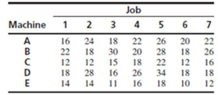
- a. Identify the blocking factor and the treatment factor.
- b. Construct an ANOVA table. You may give
ranges for the P-values. - c. Can you conclude that there are differences in costs between some pairs of machines? Explain.
- d. Which pairs of machines, if any, can you conclude, at the 5% level, to have differing mean costs?
Want to see the full answer?
Check out a sample textbook solution
Chapter 9 Solutions
STATISTICS FOR ENGINEERS+SCI.-ACCESS
Additional Math Textbook Solutions
Basic Business Statistics, Student Value Edition (13th Edition)
Business Analytics
Elementary Statistics (13th Edition)
Statistics for Business & Economics, Revised (MindTap Course List)
Introductory Statistics (10th Edition)


- Refer to Figure 8.19 Sensitivity Report for the Digital Controls, Inc. . . Intrepret the ranges of optimality for the objective funtion coefficients. Which decision variables have no limit on either the lower or upper side?arrow_forwardHow common are financial cost or contractual constraints associated with smartphone ownership? A survey of smartphone users found that 49% of the 18- to 29-year-olds, 40% of the 30- to 49-year-olds, 25% of the 50- to 64-year-olds, and 19% of those age 65 or older have reached the maximum amount of data they are allowed to use as part of their plan, at least on occasion: Suppose the survey was based on 200 smartphone owners in each of the four age groups: 18 to 29, 30 to 49, 50 to 64, and 65 and older The critical value for this test is ? (round to three decimal points as needed)arrow_forwardHow common are financial cost or contractual constraints associated with smartphone ownership? A survey of smartphone users found that 49% of the 18- to 29-year-olds, 40% of the 30- to 49-year-olds, 25% of the 50- to 64-year-olds, and 19% of those age 65 or older have reached the maximum amount of data they are allowed to use as part of their plan, at least on occasion: Suppose the survey was based on 200 smartphone owners in each of the four age groups: 18 to 29, 30 to 49, 50 to 64, and 65 and older What is the p-value?arrow_forward
- How common are financial cost or contractual constraints associated with smartphone ownership? A survey of smartphone users found that 49% of the 18- to 29-year-olds, 40% of the 30- to 49-year-olds, 25% of the 50- to 64-year-olds, and 19% of those age 65 or older have reached the maximum amount of data they are allowed to use as part of their plan, at least on occasion: Suppose the survey was based on 200 smartphone owners in each of the four age groups: 18 to 29, 30 to 49, 50 to 64, and 65 and older The test statistic is χ2STAT = ? (Round to three decimial places)arrow_forwardJensen Tire & Auto is in the process of deciding whether to purchase a maintenance contract for its new computer wheel alignment and balancing machine. Managers feel that maintenance expense should be related to usage, and they collected the following information on weekly usage (hours) and annual maintenance expense (in hundreds of dollars). Weekly Usage(hours) AnnualMaintenance Expense 19 24 16 29 26 37 34 44 38 54 23 38 30 40 37 46 46 59 44 47 -select your answer choices- b. p-value less than 0.01 between 0.01 and 0.025 between 0.025 and 0.05 between 0.05 and 0.10 greater than 0.10 Conclusion Do not conclude that there is a significant relationship between expense and weekly usage Conclude that there is a significant relationship between expense and weekly usage d. No, the expected maintenance expense is less than $3000 Yes, the expected maintenance expense is greater than $3000arrow_forwardIf a study determines the difference in average salary for subpopulations of people with blue eyes and people with brown eyes is NOT significant, then the populations of blue-eyed people and brown-eyed people are ________ different salaries. a) unlikely to have b) very unlikely to have c) guaranteed to have d) guaranteed to not havearrow_forward
- The manager of Young Corporation, wants to determine whether or not the type of work schedule for her employees has any effect on their productivity. She has selected 15 production employees at random and then randomly assigned 5 employees to each of the proposed work schedule. The following table shows the units of production(per week) under each of the work schedules. Work schedule (Treatments) Work schedule 1 Work schedule 2 Work schedule 3 50 60 70 60 65 75 70 66 55 40 54 40 45 57 55 1.State the null and alternative hypotheses to determine if there is a significant difference in the mean weekly units of production for the three types of work schedule. 2.Compute the sum of…arrow_forwardHow common are financial cost or contractual constraints associated with smartphone ownership? A survey of smartphone users found that 49% of the 18- to 29-year-olds, 37% of the 30- to 49-year-olds, 22% of the 50- to 64-year-olds, and 19% of those age 65 or older have reached the maximum amount of data they are allowed to use as part of their plan, at least on occasion: Suppose the survey was based on 200 smartphone owners in each of the four age groups: 18 to 29, 30 to 49, 50 to 64, and 65 and older. Complete parts (a) and (b) below. Use the table here to enter your data then use the TI-84 Tests. Reached Max Data 18-29 30-49 50-64 65+ Yes No Totals At the 0.05 level of significance, is there evidence of a difference among the age groups in the proportion of smartphone owners who have reached the maximum amount of data they are allowed to use as…arrow_forward(a) Show that C = 4/π.(b) Construct the Neumann method, find the expected number of trials (per one acceptance), and find the computational cost (efficiency).arrow_forward
- How common are financial cost or contractual constraints associated with smartphone ownership? A survey of smartphone users found that 48% of the 18- to 29-year-olds, 39% of the 30- to 49-year-olds, 24% of the 50- to 64-year-olds, and 19% of those age 65 or older have reached the maximum amount of data they are allowed to use as part of their plan, at least on occasion: Suppose the survey was based on 300 smartphone owners in each of the four age groups: 18 to 29, 30 to 49, 50 to 64, and 65 and older. Complete parts (a) through (c). a. At the 0.05 level of significance, is there evidence of a difference among the age groups in the proportion of smartphone owners who have reached the maximum amount of data they are allowed to use as part of their plan, at least on occasion? Find the test statistic x 2 stat? and critcal valuearrow_forwardIn a classic study of infant attachment, Harlow (1959) placed infant monkeys in cages with two artificial surrogate mothers. One “mother” was made from bare wire mesh and contained a baby bottle from which the infants could feed. The other mother was made from soft terry cloth and did not provide any access to food. Harlow observed the infant monkeys and recorded how much time per day was spent with each mother. In atypical day, the infants spent a total of 18 hours clinging to one of the two mothers. If there were no preference between the two, you would expect the time to be divided evenly, with an average of μ=9 hours for each of the mothers. However, the typical monkey spent around 15 hours per day with the terry-cloth mother, indicating a strong preference for the soft, cuddly mother. Suppose a sample of n=9 infant monkeys averaged M=15.3 hours per day with SS=216 with the terry-cloth mother. Is this result sufficient to conclude that the monkeys spent significantly more time with…arrow_forwardIn the study of evolutionary behavior, the Trivers-Willard hypothesis indicates that healthyparents should tend to have more male offspring than female, and that weaker parents should tendto have more female offspring than male. This tendency may maximize the number of each parent’sgrandchildren (and thus help to ensure that its genetic code is preserved) since a healthy maleoffspring can win many mates, but a relatively unhealthy offspring has the best chance of mating ifit is female. In an experiment to examine this hypothesis, a group of 40 opossums were monitoredand 20 of them were given an enhanced diet. After a certain period of time, the opossums with theenhanced diet had raised 19 male offspring and 14 female offspring, and the opossums without theenhanced diet had raised 15 male offspring and 15 female offspring. Does this finding provideevidence in support of the Trivers-Willard hypothesis? (a) Describe the unknown parameters ?1 and ?2. Then state the null and…arrow_forward
 MATLAB: An Introduction with ApplicationsStatisticsISBN:9781119256830Author:Amos GilatPublisher:John Wiley & Sons Inc
 Probability and Statistics for Engineering and th...StatisticsISBN:9781305251809Author:Jay L. DevorePublisher:Cengage Learning
 Statistics for The Behavioral Sciences (MindTap C...StatisticsISBN:9781305504912Author:Frederick J Gravetter, Larry B. WallnauPublisher:Cengage Learning
 Elementary Statistics: Picturing the World (7th E...StatisticsISBN:9780134683416Author:Ron Larson, Betsy FarberPublisher:PEARSON
 The Basic Practice of StatisticsStatisticsISBN:9781319042578Author:David S. Moore, William I. Notz, Michael A. FlignerPublisher:W. H. Freeman
 Introduction to the Practice of StatisticsStatisticsISBN:9781319013387Author:David S. Moore, George P. McCabe, Bruce A. CraigPublisher:W. H. Freeman