(a) Plot these points on a scatter diagram. Then estimate the regression of national income Y on the quantity of money X and plot the line on the scatter diagram. (b) How do you interpret the intercept and slope of the regression line? (c) If you had sole control over the money supply and wished to achieve a level of national income of 12.0 in 1997, at what level would you set the money supply? Explain.
(a) Plot these points on a scatter diagram. Then estimate the regression of national income Y on the quantity of money X and plot the line on the scatter diagram. (b) How do you interpret the intercept and slope of the regression line? (c) If you had sole control over the money supply and wished to achieve a level of national income of 12.0 in 1997, at what level would you set the money supply? Explain.

MATLAB: An Introduction with Applications
6th Edition
ISBN:9781119256830
Author:Amos Gilat
Publisher:Amos Gilat
Chapter1: Starting With Matlab
Section: Chapter Questions
Problem 1P

Related questions

Topic Video
Question
this is for econometrics. Please solve for #1.1 (a,b,c) #1.2, #1.3 (only a), and 1.4. Thank you! Don't use excel. Please use regular stats or cal to solve
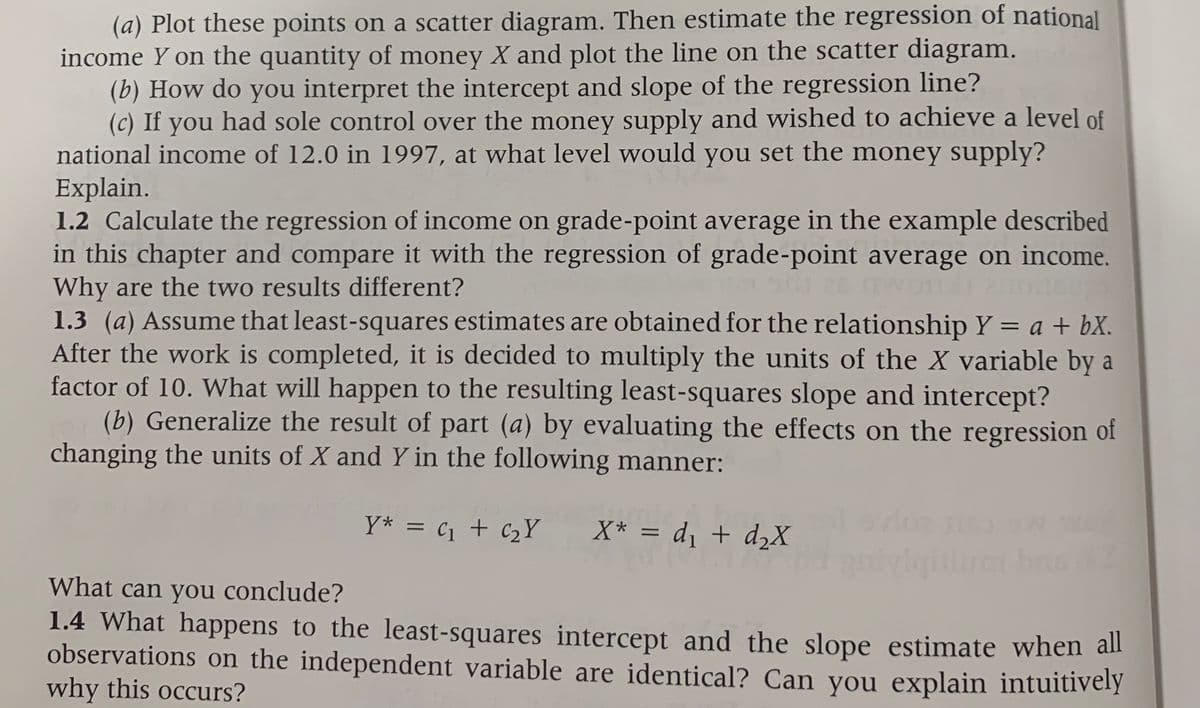
Transcribed Image Text:(a) Plot these points on a scatter diagram. Then estimate the regression of national
income Y on the quantity of money X and plot the line on the scatter diagram.
(b) How do you interpret the intercept and slope of the regression line?
(c) If you had sole control over the money supply and wished to achieve a level of
national income of 12.0 in 1997, at what level would you set the money supply?
Explain.
1.2 Calculate the regression of income on grade-point average in the example described
in this chapter and compare it with the regression of grade-point average on income.
Why are the two results different?
1.3 (a) Assume that least-squares estimates are obtained for the relationship Y = a + bX.
After the work is completed, it is decided to multiply the units of the X variable by a
factor of 10. What will happen to the resulting least-squares slope and intercept?
(b) Generalize the result of part (a) by evaluating the effects on the regression of
changing the units of X and Y in the following manner:
%3D
Y* = c1 + c2Y
X* = d, + d2X
What can you conclude?
1.4 What happens to the least-squares intercept and the slope estimate when all
observations on the independent variable are identical? Can you explain intuitively
why this occurs?
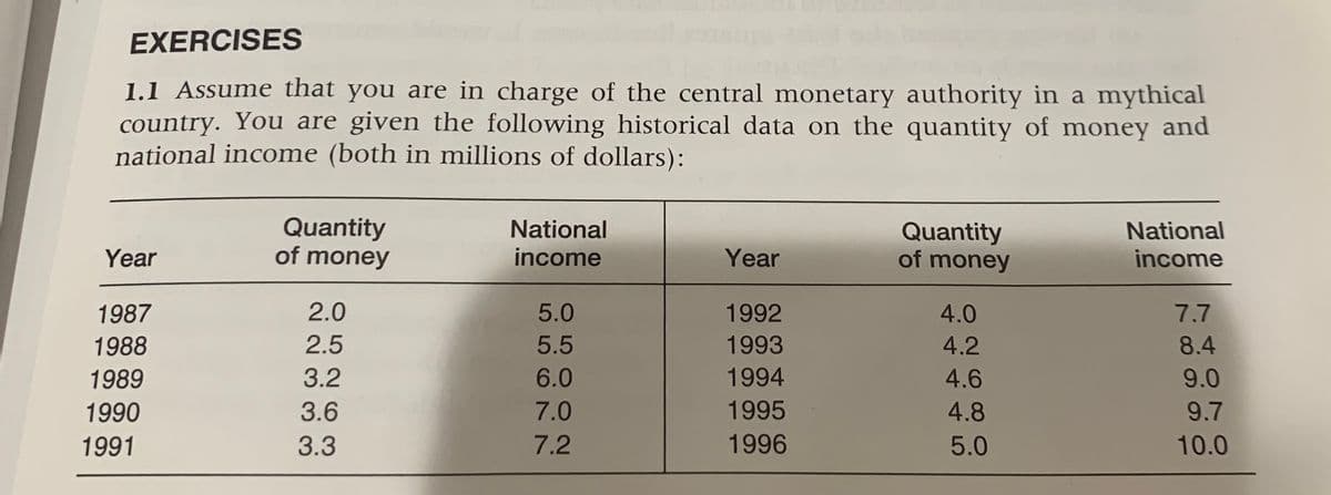
Transcribed Image Text:EXERCISES
1.1 Assume that you are in charge of the central monetary authority in a mythical
country. You are given the following historical data on the quantity of money and
national income (both in millions of dollars):
Quantity
of money
National
Quantity
of money
National
Year
income
Year
income
1987
2.0
5.0
1992
4.0
7.7
1988
2.5
5.5
1993
4.2
8.4
1989
3.2
6.0
1994
4.6
9.0
1990
3.6
7.0
1995
4.8
9.7
1991
3.3
7.2
1996
5.0
10.0
Expert Solution
This question has been solved!
Explore an expertly crafted, step-by-step solution for a thorough understanding of key concepts.

This is a popular solution!

Trending now
This is a popular solution!

Step by step
Solved in 4 steps with 1 images

Knowledge Booster


Learn more about
Need a deep-dive on the concept behind this application? Look no further. Learn more about this topic, statistics and related others by exploring similar questions and additional content below.Recommended textbooks for you
MATLAB: An Introduction with Applications
Statistics
ISBN:
9781119256830
Author:
Amos Gilat
Publisher:
John Wiley & Sons Inc

Probability and Statistics for Engineering and th…
Statistics
ISBN:
9781305251809
Author:
Jay L. Devore
Publisher:
Cengage Learning

Statistics for The Behavioral Sciences (MindTap C…
Statistics
ISBN:
9781305504912
Author:
Frederick J Gravetter, Larry B. Wallnau
Publisher:
Cengage Learning
MATLAB: An Introduction with Applications
Statistics
ISBN:
9781119256830
Author:
Amos Gilat
Publisher:
John Wiley & Sons Inc
Probability and Statistics for Engineering and th…
Statistics
ISBN:
9781305251809
Author:
Jay L. Devore
Publisher:
Cengage Learning
Statistics for The Behavioral Sciences (MindTap C…
Statistics
ISBN:
9781305504912
Author:
Frederick J Gravetter, Larry B. Wallnau
Publisher:
Cengage Learning

Elementary Statistics: Picturing the World (7th E…
Statistics
ISBN:
9780134683416
Author:
Ron Larson, Betsy Farber
Publisher:
PEARSON

The Basic Practice of Statistics
Statistics
ISBN:
9781319042578
Author:
David S. Moore, William I. Notz, Michael A. Fligner
Publisher:
W. H. Freeman

Introduction to the Practice of Statistics
Statistics
ISBN:
9781319013387
Author:
David S. Moore, George P. McCabe, Bruce A. Craig
Publisher:
W. H. Freeman