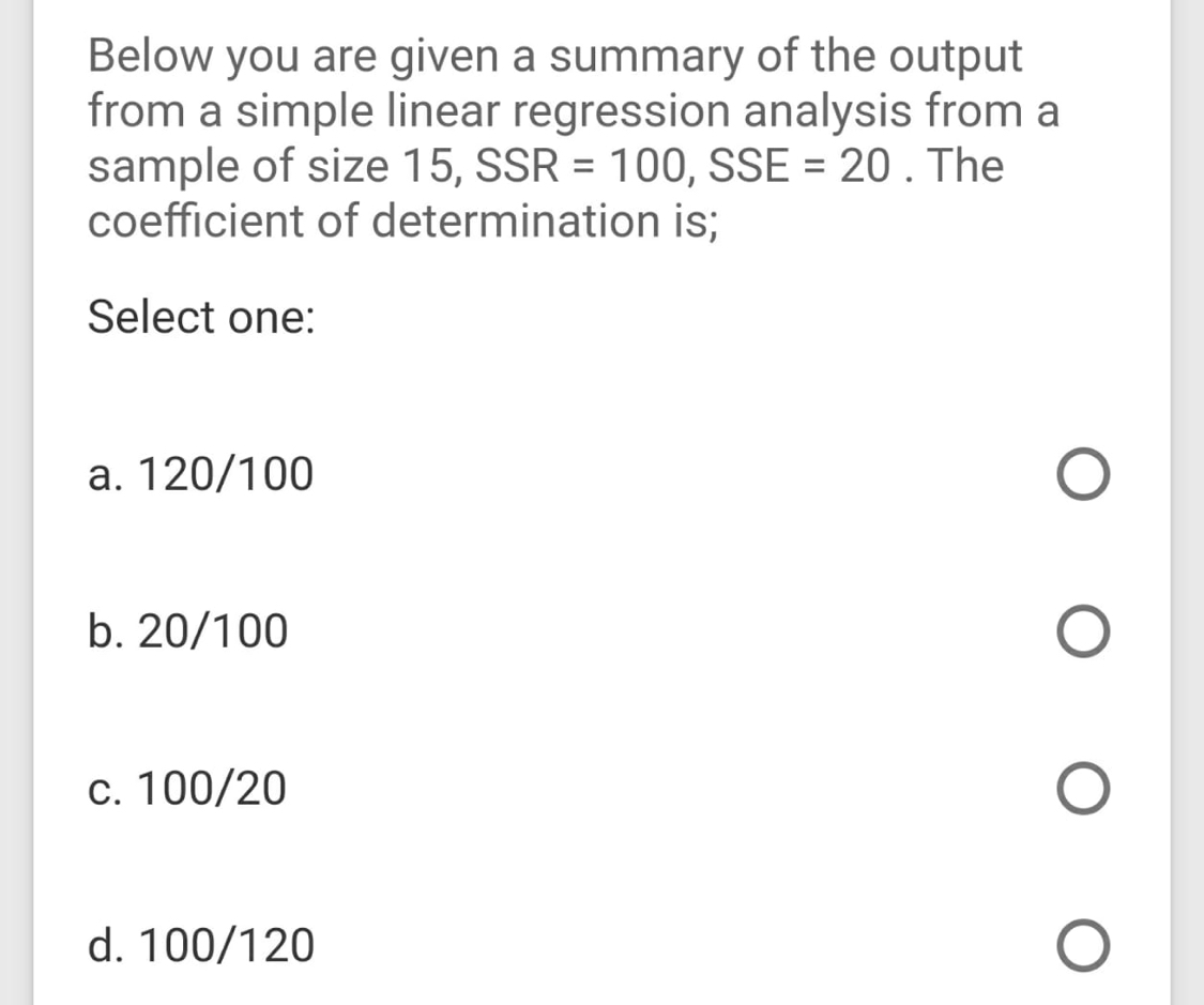
Below you are given a summary of the output from a simple linear regression analysis from a sample of size 15, SSR = 100, SSE = 20 . The coefficient of determination is;

The following regression model was fitted to sample data with 12 observations: = 30 +4.50x. What is the residual for an observation (x = 2, y = 40)? 0.50 -1 1 -0.50

The local utility company surveys 12 randomly selected customers. For each survey participant, the company collects the following: annual electric bill (in dollars) and home size (in square feet). Output from a regression analysis appears below: Bill 13.45 + 4.39*Size Coefficients Estimate Std. Error (Intercept) 13.45 Size 4.39 0.54 0.2 We are 90% confident that the mean annual electric bill increases by between dollars and dollars for every additional square foot in home size. Round your answers to three decimal places and enter in increasing order.

The table below gives the number of weeks of gestation and the birth weight (in pounds) for a sample of five randomly selected babies. Using this data, consider the equation of the regression line, y = bo + b1x, for predicting the birth weight of a baby based on the number of weeks of gestation. Keep in mind, the correlation coefficient may or may not be statistically significant for the data given. Remember, in practice, it would not be appropriate to use the regression line to make a prediction if the correlation coefficient is not statistically significant. Weeks of Gestation 33 34 36 38 41 Weight (in pounds) 6 6.1 6.8 7.3 7.9 Table Copy Data Step 4 of 6: Find the estimated value of y when x = 36. Round your answer to three decimal places.

Listed below are systolic blood pressure measurements (in mm Hg) obtained from the same woman. Find the regression equation, letting the right arm blood pressure be the predictor (x) variable. Find the best predicted systolic blood pressure in the left arm given that the systolic blood pressure in the right arm is 80 mm Hg. Use a significance level of 0.05. Right Arm 100 99 93 77 77 Q Left Arm 174 168 148 148 146 Click the icon to view the critical values of the Pearson correlation coefficient r The regression equation is ŷ=+x. (Round to one decimal place as needed.) mm Hg. Given that the systolic blood pressure in the right arm is 80 mm Hg, the best predicted systolic blood pressure in the left arm is (Round to one decimal place as needed.) Data table Critical Values of the Pearson Correlation Coefficient r α = 0.05 α = 0.01 0.950 0.990 0.959 0.878 0.811 0.917 0.754 0.875 0.707 0.834 0.666 0.798 0.632 0.765 0.602 0.735 0.576 0.708 0.553 0.684 0.532 0.661 0.514 0.641 0.497 0.623 0.482…

The statistic used to test whether individual regression coefficients are different from zero in the population is: Select one: a. F O b. b Oc. R2 O d. t Clear my choice

The value of PRESS for five different regression models are A = 42.3, B = 47.4, C = 51.5, D =40.6, and E = 54.6. Based only on this statistic, which model is preferred?

The correlation between two variables x and y is –0.6. If we used a regression line to predict y using x, what percent of the variation in y would be explained?