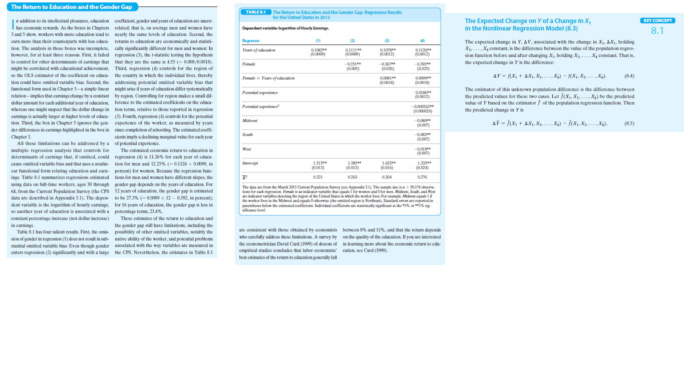
The Return to Education and the Gender Gap TABLE 8.1 The Return to Education and the Gender Gap: Regression Results for the United States In 2012 The Expected Change on Y of a Change In X, In the Nonlinear Regresslon Model (8.3) n addition to its intellectual pleasures, education coefficient, gender and years of education are uncor- KEY CONCEPT has economic rewards. As the boxes in Chapters related; that is, on average men and women have 3 and 5 show, workers with more education tend to nearly the same levels of education. Second, the Dapandent varlables: logarithm of Hourly Eamings. 8.1 earn more than their counterparts with less educa- returns to education are economically and statisti- Regressor (1) (2) 3) (4) The expected change in Y, AY, associated with the change in X1, AX1, holding X2, ..., Xg constant, is the difference between the value of the population regres- sion function before and after changing X1, holding X2, ..., Xg constant. That is, the expected change in Y is the difference: tion. The analysis in those boxes was incomplete, cally significantly different for men and women: In however, for at least three reasons. First, it failed regression (3), the t-statistic testing the hypothesis 0.1078 (0.0012) 0 1082 0.1126** (0.0012) Years of education 0.1111* (0.0009) (0.0009) to control for other determinants of earnings that that they are the same is 4.55 (- 0.008/0.0018). might be correlated with educational achievement, Third, regression (4) controls for the region of -0251 (0.005) -0.367 (0.026) -0.392 (0.025) Female so the OLS estimator of the coefficient on educa- the country in which the individual lives, thereby AY = f(X1 + AX1, X2, . .., X2) – fX1, X2, ..., Xx). (8.4) 0.0081 (0.0018) 0,0099 (0.0018) Female x Years of education tion could have omitted variable bias. Second, the addressing potential omitted variable bias that functional form used in Chapter 5-a simple linear might arise if years of education differ systematically The estimator of this unknown population difference is the difference between the predicted values for these two cases. Let f(X1, X2, -.., Xg) be the predicted value of Y based on the estimator f of the population regression function. Then the predicted change in Y is L0186 (0.0012) Potential experience relation-implies that earnings change by a constant by region. Controlling for region makes a small dif- ...... dollar amount for each additional year of education, ference to the estimated coefficients on the educa- whereas one might suspect that the dollar change in tion terms, relative to those reported in regression Potential experience -0.000063* (0.00X0024) earnings is actually larger at higher levels of educa- (3). Fourth, regression (4) controls for the potential tion. Third, the box in Chapter 5 ignores the gen- experience of the worker, as measured by years Midwest -0.080* AỸ = f(x, + AX, Xg, ...,X) - (X1, X2, - .., X2). (8.5) (0.007) der differences in earnings highlighted in the box in since completion of schooling. The estimated coeffi- South -0.063 Chapter 3. All these limitations can be addressed by a of potential experience. multiple regression analysis that controls for determinants of earnings that, if omitted, could regression (4) is 11.26% for each year of educa- cause omitted variable bias and that uses a nonlin- tion for men and 12.25% (- 0.1126 + 0.0099, in cients imply a declining marginal value for each year (0.007) The estimated economic return to education in West -0.018** (0.007) Intercept 1515* 1.585** 1.632* 1.335* (0.013) (0.013) (0.016) (0.024) ear functional form relating education and earn- percent) for women. Because the regression func- ings. Table 8.1 summarizes regressions estimated tions for men and women have different slopes, the 0.221 0263 0.264 0.276 using data on full-time workers, ages 30 through gender gap depends on the years of education. For The data are from the March 2013 Current Population Survey (see Appendix 31). The sample size is a = 50,174 observa- tions for each rearesion. Female is an indicator variable that equals 1 for women and 0 for men. Midwert, South, and West are indicator variables denoting the region of the United States in which the worker lives For example, Midwat oquals 1 if the worker lives in the Midwest and equals O otherwise (the omitted region is Northeast). Standard errors are reported in parentheses below the estimated coefficients. Individual coefficients are statistically significant at the *5% or **1% sig- nificance level. 64, from the Current Population Survey (the CPS 12 years of education, the gender gap is estimated data are described in Appendix 3.1). The depen- to be 27.3% (- 0.0099 x 12 – 0.392, in percent); dent variable is the logarithm of hourly earnings, for 16 years of education, the gender gap is less in so another year of education is associated with a percentage terms, 23.4%. constant percentage increase (not dollar increase) These estimates of the return to education and the gender gap still have limitations, including the in earnings. able 8.1 has four salient results. First, the omis- possibility of other omitted variables, notably the are consistent with those obtained by economists between 8% and 11%, and that the return depends who carefully address these limitations. A survey by on the quality of the education. If you are interested sion of gender in regression (1) does not result in sub- native ability of the worker, and potential problems stantial omitted variable bias: Even though gender associated with the way variables are measured in enters regression (2) significantly and with a large the CPS. Nevertheless, the estimates in Table 8.1 the econometrician David Card (1999) of dozens of in learning more about the economic return to edu- empirical studies concludes that labor economists cation, see Card (1999). best estimates of the return to education generally fall


Read the box “The Return to Education and the Gender Gap”.
a. Consider a man with 16 years of education and 2 years of experience
who is from a western state. Use the results from column (4)
of Table 8.1 and the method in Key Concept 8.1 to estimate the
expected change in the logarithm of average hourly earnings (AHE)
associated with an additional year of experience.
b. Repeat (a), assuming 10 years of experience.
c. Explain why the answers to (a) and (b) are different.
d. Is the difference in the answers to (a) and (b) statistically significant
at the 5% level? Explain.
e. Would your answers to (a) through (d) change if the person were a
woman? If the person were from the South? Explain.
f. How would you change the regression if you suspected that the effect
of experience on earnings was different for men than for women?


Trending now
This is a popular solution!

Step by step
Solved in 5 steps with 7 images

Can you also provide solutions for question d,e, and f?
d. Is the difference in the answers to (a) and (b) statistically significant
at the 5% level? Explain.
e. Would your answers to (a) through (d) change if the person were a
woman? If the person were from the South? Explain.
f. How would you change the regression if you suspected that the effect
of experience on earnings was different for men than for women?


