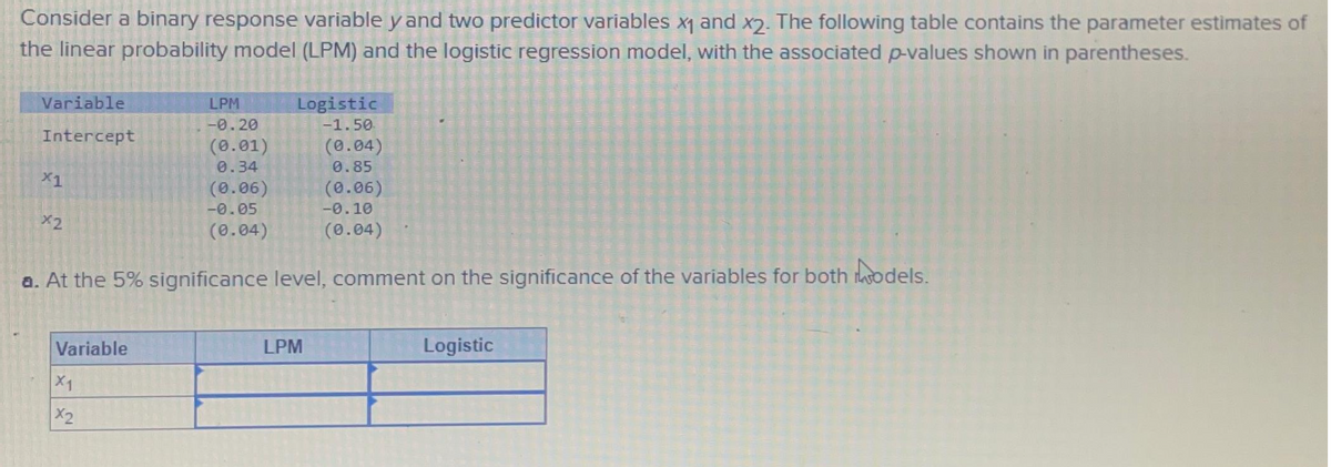
Consider a binary response variable y and two predictor variables x₁ and x2. The following table contains the parameter estimates of the linear probability model (LPM) and the logistic regression model, with the associated p-values shown in parentheses. Variable Intercept Logistic -1.50 (0.04) 0.85 (0.06) -0.10 (0.04) a. At the 5% significance level, comment on the significance of the variables for both Models. x1 x2 Variable LPM -0.20 (0.01) 0.34 X1 X2 (0.06) -0.05 (0.04) LPM Logistic

Q9 The explanatory variable in linear correlation/regression model is recorded on which of thesemeasurement scales: A. categorical B. ordinal C. quantitative D. none of the above

Consider the following correlations -0.9 , -0.5 , -0.2 , 0 , 0.2 , 0.5  and 0.9. For each give the fraction of the variation in y that is explained by the least-squares regression of y on x.

q13

In a study investigating maternal risk factors for congenital syphilis, syphilis is treated as a binary outcome variable, where 1 represents the presence of disease in a newborn and 0 represents absence of disease. The estimated coefficients from a logistic regression model containing the predictors cocaine or crack use, marital status, number of prenatal visits to a doctor, alcohol use and level of education are included in the table below. The estimated intercept is not included in the table. a. As an expectant mother’s number of prenatal visits to the doctor increases, does the probability that her child will be born with congenital syphilis increase or decrease?b. Marital status is a binary variable, where 1 indicates that a woman is unmarried and 0 indicates that she is married. What are the estimated relative odds that a newborn will suffer from syphilis for unmarried versus married mothers after holding the other variables in the model constant?c. Cocaine or crack use is also a…

Let's study the relationship between brand, camera resolution, and internal storage capacity on the price of smartphones. Use α = .05 to perform a regression analysis of the Smartphones01CS dataset, and then answer the following questions. When you copy and paste output from MegaStat to answer a question, remember to choose to "Keep Formatting" to paste the text. a. Did you find any evidence of multicollinearity and variance inflation among the predictors. Explain your answer using a VIF analysis. b. Copy and paste the normal probability plot for your analysis. Is there any evidence that the errors are not normally distributed? Explain. c. Copy and paste the Residuals vs. Predicted Y-values. Does the pattern support the null hypothesis of constant variance for the errors? Explain. d. Study the residuals analysis. Which observations, if any, have unusual residuals? e. Study the residuals analysis. Calculate the leverage statistic. Which observations, if any, are high leverage…

randomly selected middle school students. Using this data, consider the equation of the regression line, yˆ=b0+b1x, for predicting the overall grade average for a middle school student based on the number of hours spent unsupervised each day. Keep in mind, the correlation coefficient may or may not be statistically significant for the data given. Remember, in practice, it would not be appropriate to use the regression line to make a prediction if the correlation coefficient is not statistically significant. Hours Unsupervised 1.5 2 3 3.5 4 4.5 5.5 Overall Grades 99 96 84 75 68 65 60 Table   Step 1 of 6 :  Find the estimated slope. Round your answer to three decimal places.