
Related questions
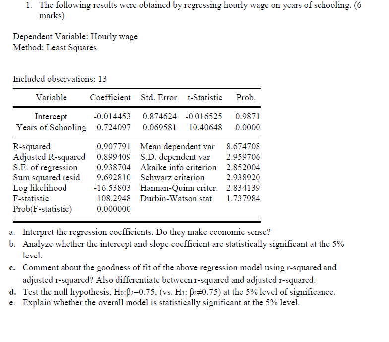
The following results were obtained by regressing mean hourly wage in dollars (Y) on years of schooling (X).
|
Dependent Variable: MEAN_WAGE |
|
|
||||||
|
Method: Least Squares |
|
|
||||||
|
Date: 02/15/15 Time: 11:11 |
|
|
||||||
|
Sample: 1 13 |
|
|
|
|||||
|
Included observations: 13 |
|
|
||||||
|
|
|
|
|
|
|
|||
|
|
|
|
|
|
|
|||
|
Variable |
Coefficient |
Std. Error |
t-Statistic |
Prob. |
|
|||
|
|
|
|
|
|
|
|||
|
|
|
|
|
|
|
|||
|
C |
-0.014453 |
0.874624 |
-0.016525 |
0.9871 |
|
|||
|
YEARS_SCHOOLING |
0.724097 |
0.069581 |
10.40648 |
0.0000 |
|
|||
|
|
|
|
|
|
|
|||
|
|
|
|
|
|
|
|||
|
R-squared |
0.907791 |
Mean dependent var |
8.674708 |
|
||||
|
Adjusted R-squared |
0.899409 |
S.D. dependent var |
2.959706 |
|
||||
|
S.E. of regression |
0.938704 |
Akaike info criterion |
2.852004 |
|
||||
|
Sum squared resid |
9.692810 |
Schwarz criterion |
2.938920 |
|
||||
|
Log likelihood |
-16.53803 |
Hannan-Quinn criter. |
2.834139 |
|
||||
|
F-statistic |
108.2948 |
Durbin-Watson stat |
1.737984 |
|
||||
|
Prob(F-statistic) |
0.000000 |
|
|
|
|
|||
|
|
|
|
|
|
|
|||
|
|
|
|
|
|
|
|||
|
|
|
|
|
|
|
|||
- Interpret the regression coefficients. Do they make economic sense?
- Would you conclude that there is a statistically significant relationship at the 5% level between mean hourly wage (Y) and years of schooling (X)? (Hint: Test H0: β2=0)
- Comment about the goodness of fit of the above regression model?
- Test the null hypothesis, H0:β2=1, (vs. H1: β2≠1) at the 1% level of significance.


Step by stepSolved in 3 steps


- A research team conducted a study of VARIABILITY in students' test performance. Researchers assume that individual records are normally distributed with unknown mean and variance. They collected a sample of n = 25 test scores with summaries shown below. Sample Mean = X = 75.2 and Sample SD = S = 15 1. At the significance level, a = 0.01, do researchers have sufficient evidence that the POPULATION VARIANCE would be ABOVE 120? • Show critical value • Evaluate Test Statistic • Formulate Rejection Rule • State your decision 2. At the significance level, a = 0.01, do researchers have sufficient evidence that the POPULATION VARIANCE would be BELOW 540? • Show critical value • Evaluate Test Statistic • Formulate Rejection Rule • State your decision Solutionarrow_forwardsolve for image and find critical valuesarrow_forwardThe mean ±1 sd of ln [calcium intake (mg)] among 25 females, 12 to 14 years of age, below the poverty level is 6.56 ± 0.64. Similarly, the mean ± 1 sd of ln [calcium intake (mg)] among 40 females, 12 to 14 years of age, above the poverty level is 6.80 ± 0.76. 8.2 Test for a significant difference between the variances of the two groups. Find the P value. Do not use excell. Solve the step by steparrow_forward
- The mean time it takes a crew to restart an aluminum rolling mill after a failure is of interest. The crew was observed over 25 occasions, and the results were mean = 26 minutes and variance = 12 minutes. If repair time is normally distributed, (a) Find a 95% confidence interval on the true but unknown mean repair time. (b) Test the hypothesis that the true mean repair time is 30 minutes.arrow_forward0.6.3 Question 3 Is the cubic effect significant? How about quadratic and linear effects? Analysis of Variance Table Response: EX Df Sum Sq Mean Sq F value Pr(>F) MET 1 332 332 0.1246 0.7257742 I(MET^2) 1 37504 37504 14.0572 0.0005141 *** I(MET^3) 1 7245 7245 2.7154 0.1065086 Residuals 44 117390 2668 > anova(quadModel) Analysis of Variance Table Response: EX Df Sum Sq Mean Sq F value Pr(>F) MET 1 332 332 0.120 0.7306134 I(MET^2) 1 37504 37504 13.541 0.0006216 *** Residuals 45 124635 2770 --- Signif. codes: 0 ‘***’ 0.001 ‘**’ 0.01 ‘*’ 0.05 ‘.’ 0.1 ‘ ’ 1arrow_forwarduse the date form the second picture to answer question 3 please help me with question 3arrow_forward
- An excess of high values for the cases distributed on a graph results in a positive skew in the data?arrow_forwardThe maximum weights (in kilograms) for which one repetition of a half squat can be performed and the times (in seconds) to run a 10-meter sprint for 12 international soccer players are shown in the attached data table with a sample correlation coefficient r of -0.971. A 13th data point was added to the end of the data set for an international soccer player who can perform the half squat with a maximum of 210 kilograms and can sprint 10 meters in 2.01 seconds. Describe how this affects the correlation coefficient r. Use technology. Click the icon to view the data set. The new correlation coefficient r going from -0.971 to (Round to three decimal places a gets stronger, gets weaker, stays the same,arrow_forward
- MATLAB: An Introduction with ApplicationsStatisticsISBN:9781119256830Author:Amos GilatPublisher:John Wiley & Sons Inc
 Probability and Statistics for Engineering and th...StatisticsISBN:9781305251809Author:Jay L. DevorePublisher:Cengage Learning
 Statistics for The Behavioral Sciences (MindTap C...StatisticsISBN:9781305504912Author:Frederick J Gravetter, Larry B. WallnauPublisher:Cengage Learning
  Elementary Statistics: Picturing the World (7th E...StatisticsISBN:9780134683416Author:Ron Larson, Betsy FarberPublisher:PEARSON
 The Basic Practice of StatisticsStatisticsISBN:9781319042578Author:David S. Moore, William I. Notz, Michael A. FlignerPublisher:W. H. Freeman
 Introduction to the Practice of StatisticsStatisticsISBN:9781319013387Author:David S. Moore, George P. McCabe, Bruce A. CraigPublisher:W. H. Freeman