
MATLAB: An Introduction with Applications
6th Edition
ISBN: 9781119256830
Author: Amos Gilat
Publisher: John Wiley & Sons Inc
expand_more
expand_more
format_list_bulleted
Related questions
Concept explainers
Question
(b) For the
(x, y)
data set of part (a), compute the equation of the sample least-squares line
ŷ = a + bx.
(Use 4 decimal places.)
| a | |
| b |
If the number of hits was
9.1 (× 105)
one day, what do you predict for the number of hits the next day? (Use 1 decimal place.)
(× 105) hits
(c) Compute the sample
r2.
(Use 4 decimal places.)
| r | |
| r2 |
Test
ρ > 0
at the 1% level of significance. (Use 2 decimal places.)
| t | |
| critical t |
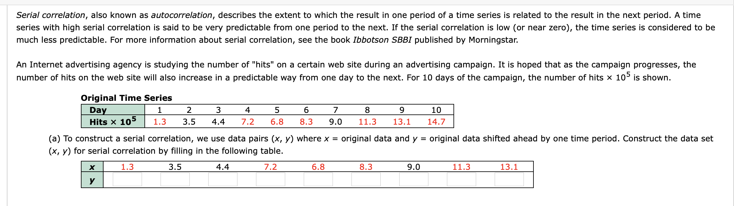

Transcribed Image Text:Serial correlation, also known as autocorrelation, describes the extent to which the result in one period of a time series is related to the result in the next period. A time
series with high serial correlation is said to be very predictable from one period to the next. If the serial correlation is low (or near zero), the time series is considered to be
much less predictable. For more information about serial correlation, see the book Ibbotson SBBI published by Morningstar.
An Internet advertising agency is studying the number of "hits" on a certain web site during an advertising campaign. It is hoped that as the campaign progresses, the
number of hits on the web site will also increase in a predictable way from one day to the next. For 10 days of the campaign, the number of hits x 105 is shown.
Original Time Series
Day
Hits x 105
2
4
9.
10
1.3
3.5
4.4
7.2
6.8
8.3
9.0
11.3
13.1
14.7
(a) To construct a serial correlation, we use data pairs (x, y) where x =
(x, y) for serial correlation by filling in the following table.
original data and y = original data shifted ahead by one time period. Construct the data set
%D
х
1.3
3.5
4.4
7.2
6.8
8.3
9.0
11.3
13.1
Expert Solution
This question has been solved!
Explore an expertly crafted, step-by-step solution for a thorough understanding of key concepts.

This is a popular solution

Trending nowThis is a popular solution!

Step by stepSolved in 2 steps with 2 images

Knowledge Booster


Learn more about
Need a deep-dive on the concept behind this application? Look no further. Learn more about this topic, statistics and related others by exploring similar questions and additional content below.Similar questions
- In a regression study, relating Price/unit (x) to Weekly Sales (in Kg.), with the scatter plot showing a strong negative direction, 63% of the variability in sales could be accounted for by the variation in the Unit Price. The correlation coefficient in this study is: 0.7 -0.4 -0.79 0.4arrow_forwardc) Show that the coefficient of determination, R², can also be obtained as the squared correlation between actual Y values and the Y values estimated from the regression model where Y is the dependent variable. Note that the coefficient of correlation between Y and X is Eyixi r = And also that ỹ = ŷ (18.75)arrow_forwardThe regression equation is: ŷ = 67.16 + 8.417x where ŷ is the miles traveled, and x is the MPG. The sample size used was all 110 MPG records. The correlation coefficient r = 0.620. Use the information to obtain an estimate of my mileage if my MPG is 22. Is it option: a.) cannot estimate ŷ rcrit = 0.195; the correlation IS NOT significant b.) ŷ = 252.33 rcrit = 0.195; the correlation IS significant c.) ŷ = 252.33 rcrit = 0.187; the correlation IS significant d.) cannot estimate ŷ rcrit = 0.187; the correlation IS NOT significantarrow_forward
- A movie studio wishes to determine the relationship between the revenue from rental of comedies on streaming services and the revenue generated from the theatrical release of such movies. The studio has the following bivariate data from a sample of fifteen comedies released over the past five years. These data give the revenue x from theatrical release (in millions of dollars) and the revenue y from streaming service rentals (in millions of dollars) for each of the fifteen movies. Also shown are the scatter plot and the least-squares regression line for the data. The equation for this line is y = 3.58 +0.15x. Theater revenue, x (in millions of dollars) 26.4 36.7 43.5 31.6 60.4 14.8 21.3 49.3 7.7 24.8 27.8 12.9 60.6 26.4 66.4 Send data to calculator V Rental revenue, y (in millions of dollars) 8.1 12.4 6.8 5.1 15.4 2.6 5.8 16.5 2.2 9.1 3.3 9.8 10.8 11.7 9.6 Based on the studio's data and the regression line, complete the following. Rental revenue in millions of dollars) 0 X 10 X 20…arrow_forwardAn ecologist is interested in exploring the relationship between pollination rate and the number of bees present at apple orchards. The relationship is: (Pollination rate) = 372.6 + 13.5 x (bees) with r = 0.80. The best interpretation of the correlation coefficient is: (pick one) 1. 64% of the variability in pollination rate observed at apple orchards is explained by the relationship with the number of bees 2. the correlation between pollination rate and number of bees is 0.64 3. 80% of the variability in number of bees at apple orchards is explained by the relationship with the pollination rate 4. the correlation between pollination rate and number of bees is 0.80arrow_forwardIn a regression study, relating Price/unit (x) to Weekly Sales (in Kg.), with the scatter plot showing a strong negative direction, 63% of the variability in sales could be accounted for by the variation in the Unit Price. The correlation coefficient in this study is: 0.79 -0.4 -0.79 0.4arrow_forward
- What information is provided by r2? What are the primary uses of partial correlations?arrow_forwardA nutritionist collects data from 25 popular breakfast cereals. For each cereal, the number of calories per serving is plotted on the x-axis against the number of milligrams of sodium on the y-axis. The value of r for the resulting scatterplot is 0.83. How would the value of the correlation coefficient, r, change if sodium was plotted on the x-axis and calories plotted on the y-axis? The value of r would increase. The value of r would not change. The value of r would change to –0.83. The value of r could increase or decrease, depending of the strength of the new relationship.arrow_forwardhow can i calculatearrow_forward
arrow_back_ios
arrow_forward_ios
Recommended textbooks for you
- MATLAB: An Introduction with ApplicationsStatisticsISBN:9781119256830Author:Amos GilatPublisher:John Wiley & Sons Inc
 Probability and Statistics for Engineering and th...StatisticsISBN:9781305251809Author:Jay L. DevorePublisher:Cengage Learning
 Statistics for The Behavioral Sciences (MindTap C...StatisticsISBN:9781305504912Author:Frederick J Gravetter, Larry B. WallnauPublisher:Cengage Learning
  Elementary Statistics: Picturing the World (7th E...StatisticsISBN:9780134683416Author:Ron Larson, Betsy FarberPublisher:PEARSON
 The Basic Practice of StatisticsStatisticsISBN:9781319042578Author:David S. Moore, William I. Notz, Michael A. FlignerPublisher:W. H. Freeman
 Introduction to the Practice of StatisticsStatisticsISBN:9781319013387Author:David S. Moore, George P. McCabe, Bruce A. CraigPublisher:W. H. Freeman
MATLAB: An Introduction with Applications
Statistics
ISBN:9781119256830
Author:Amos Gilat
Publisher:John Wiley & Sons Inc
Probability and Statistics for Engineering and th...
Statistics
ISBN:9781305251809
Author:Jay L. Devore
Publisher:Cengage Learning
Statistics for The Behavioral Sciences (MindTap C...
Statistics
ISBN:9781305504912
Author:Frederick J Gravetter, Larry B. Wallnau
Publisher:Cengage Learning
Elementary Statistics: Picturing the World (7th E...
Statistics
ISBN:9780134683416
Author:Ron Larson, Betsy Farber
Publisher:PEARSON
The Basic Practice of Statistics
Statistics
ISBN:9781319042578
Author:David S. Moore, William I. Notz, Michael A. Fligner
Publisher:W. H. Freeman
Introduction to the Practice of Statistics
Statistics
ISBN:9781319013387
Author:David S. Moore, George P. McCabe, Bruce A. Craig
Publisher:W. H. Freeman