
Related questions
In this question, we want to analyse the total energy production in Australia on a monthly basis from 2010 to 2022. The energy production is measured in gigawatt-hours (GWh). This covers a
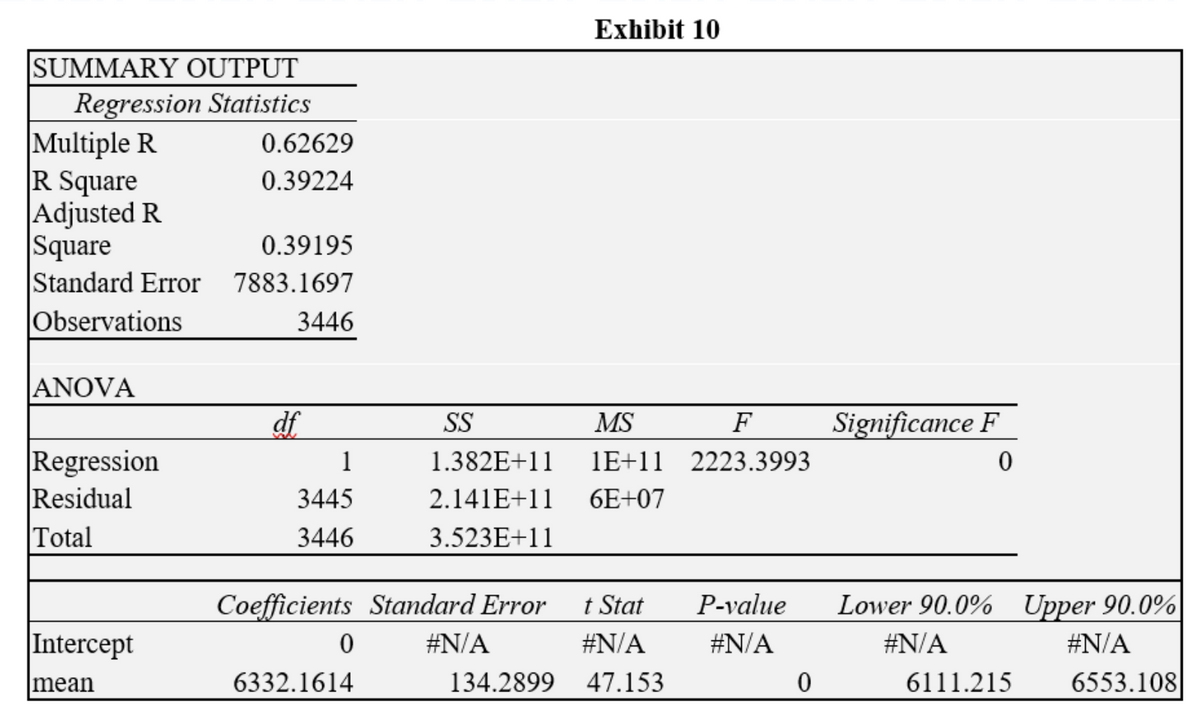
a) To analyse the energy production, we start by defining the following variables:
total_prod = is the total monthly energy production from different sources (GWh)
Exhibit 10 below shows the regression output from a regression of total_prod (dependent variable) on Mean (independent variable):
i) What does the coefficient of the “mean” value tell us?
ii) State and in the context, interpret the 90% confidence interval for the “Australia energy production”.


Trending nowThis is a popular solution!

Step by stepSolved in 3 steps with 1 images


- Accounting Today identified the top accounting firms in 10 geographic regions across the United States. All 10 regions reported growth in 2014. The Southeast and Gulf Coast regions reported growth of 12.36% and 5.8%, respectively. A characteristic description of the accounting firms in the Southeast and Gulf Coast regions included the number of partners in the firm. The file AccountingPartners3 contains the number of partners. (Data extracted from bit.ly/1BoMzsv) Assuming that the population variances from both offices are equal, at the 0.10 level of significance, is there evidence of a difference between Southeast region accounting firms and Gulf Coast accounting firms with respect to the mean number of partners? Referring to Table 10-1, the proper conclusion for this test is Question 5 options: 1) at the α = 0.10 level, there is sufficient evidence to indicate a difference in the mean time to clear problems in the two offices.…arrow_forwardThe demand and forecast information for the XYZ Company over a twelve-month period has been collected in the Microsoft Excel Online file below. Use the Microsoft Excel Online file below to develop forecast accuracy and answer the following questions. Forecast Accuracy Measures Period Actual Demand Forecast Error Absolute Error Error^2 Abs. % Error 1 1,300 1,378 2 2,000 1,676 3 1,800 1,974 4 1,700 2,272 5 2,300 2,570 6 3,800 2,868 7 3,200 3,166 8 3,100 3,464 9 3,900 3,761 10 4,600 4,059 11 4,200 4,357 12 4,300 4,655 Total Average RSFE MAD MSE MAPE Tracking Signal 1. What can be concluded about the quality of the forecasts? Assume that the control limit for the tracking signal is ±3. The results indicate (bias or no bias) in the…arrow_forwardA method of estimating earth temperature based on local precipitation is to build models based on 100s of years of earth at several different constant green house gas level (So constant global temperature for 100s of years) , and compare the correlation of statistical relationships between predicted precipitation patterns in a region, and observed precipitation patterns for a region in a few year time period.arrow_forward
- Ims.tu.edu.sa قائمة القراءة. Remaining Time: 34 minutes, 24 seconds. v Question Completion Status: QUESTION 1 "Suppose X has an exponential distribution with ß=1/2 , then P (X2 2) is " 0.3988 O 0.0183 0.4786 O 0.2916 QUESTION 2 "Suppose X has an exponential distribution with ß=1/4 , then P (Xs1.) is " O 0.9817 O 0.3246 O 0.4105 O 0.5116 QUESTION 3arrow_forwardChlorophylls a and b are plant pigments that absorb sunlight and transfer the energy into photosynthesis of carbohydrates from CO2 and H2O, releasing O2 in the process. Chlorophylls were extracted from chopped up grass and measured by spectrophotometry. The table shows results for chlorophyll a for four separate analysis of five blades of grass. Chlorophyll a (g/L) Blade 1 Blade 2 Blade 3 Blade 4 Blade 5 1.09 1.26 1.1 1.23 0.85 0.86 0.96 1.21 1.3 0.65 0.93 0.8 1.27 0.97 0.86 0.99 0.73 1.12 0.97 1.03 Four replicate measurements for each blade of grass tell us the precision of the analytical procedure (sanalysis). Differences between mean values for each of the five blades of grass are a measure of variation due to sampling (ssampling). Using Excel and it’s ANOVA function, find the standard deviations attributable to sampling and to analysis, as well as the overall standard deviation arising from both sources.arrow_forwardResearch was belng conducted on whether a new diet wll help reduce a person's cholesterol level. The doctor randomly selected some of his patients and recorded their cholesterol levels before and after completing the dlet. The data is gven below. Test the claim that the dlet Is effective In reducing a person's cholesterol level at the a 0.05 level of significance. Patlent C. Cholesterol Level Before 209 210 205 198 216 217 238 Diet Cholesterol Level After 200 198 197 196 214 211 222 Diet Calculator Function [ Select ] P-Value [ Select ]arrow_forward
- Please submit one excel file with answer cells that require formulas having the formulas within the cell. A manager is trying to educate employees on the effects of personal health and workplace performance. The manager has gathered data from a group of employees to evaluate the effects of sleep and sickness. The manager asked employees to record the total number of hours of sleep they had over 10 working days in two weeks and compared it to the number of sick days that each took over those 10 days. Sick Days Total hours of sleep 0 80 2 40 1 60 0 70 3 50 2 90 4 35 1 68 0 72 2 55 Is the model statistically significant at the .05 level? How much of the variability in sick days is determined by hours of sleep? PLEASE PUT THE ANSWER IN AN EXCEL FILE WITH THE FORMULAS SHOWN PLEASE USE AN EXCEL FILE.arrow_forward(b) Table 1 shows consumables usage data from a leading manufacturer. Forecast the demand for August, September and October using: i) a three-month moving average ii) a four-month weighted moving average using 50 percent of the actual usage for the most recent month, 20 percent of two months ago, 15 percent of three months ago and 15 percent of four months ago. Using an example, explain what are the benefits of using the weighted moving average method of forecasting instead? Month February 2023 March 2023 April 2023 May 2023 June 2023 July 2023 Consumables Used 884 892 972 990 956 880arrow_forwardLOG Take Test Unit 3 Test d.com/webapps/assessment/take/launch.jsp?course_assessment_id=_415098_1&course_id=_309271_1&new.... Remaining Time: 4 hours, 44 minutes, 03 seconds. Qu Browse Local Files QUESTION 13 Status: A state lottery draws six numbers between 1 and 63. If you wanted to buy every combination possible, how many combinations are there? QUESTION 14 Match each scenario with the counting rule that would be used to solve it. 5 point 4 poinarrow_forward
- MATLAB: An Introduction with ApplicationsStatisticsISBN:9781119256830Author:Amos GilatPublisher:John Wiley & Sons Inc
 Probability and Statistics for Engineering and th...StatisticsISBN:9781305251809Author:Jay L. DevorePublisher:Cengage Learning
 Statistics for The Behavioral Sciences (MindTap C...StatisticsISBN:9781305504912Author:Frederick J Gravetter, Larry B. WallnauPublisher:Cengage Learning
  Elementary Statistics: Picturing the World (7th E...StatisticsISBN:9780134683416Author:Ron Larson, Betsy FarberPublisher:PEARSON
 The Basic Practice of StatisticsStatisticsISBN:9781319042578Author:David S. Moore, William I. Notz, Michael A. FlignerPublisher:W. H. Freeman
 Introduction to the Practice of StatisticsStatisticsISBN:9781319013387Author:David S. Moore, George P. McCabe, Bruce A. CraigPublisher:W. H. Freeman