Chapter 10, Problem 3CS

To determine

Explain whether it is possible that the gender is independent of department at the level of significance of $\alpha =0.01$.

Answer to Problem 3CS

There is enough evidence to conclude that the gender differs among departments.

Explanation of Solution

Calculation:

The contingency table 10.11 with 2 rows and 6 columns are given. The two rows consist of gender and the six columns consist of six departments.

Contingency table:

A contingency table is obtained as using two qualitative variables. One of the qualitative variable is row variable that has one category for each row of the table another is column variable has one category for each column of the table.

Step 1:

The hypotheses are:

Null Hypothesis:

$H_0:\text{The gender and departments are independent}\text{.}$

That is, the gender does not differ among departments.

Alternate Hypothesis:

$H_1:\text{The gender and departments are not independent}.$

That is, the gender differs among departments.

Step 2:

Now, it is obtained that,

Department	A	B	C	D	E	F	Row Total
Male	825	560	325	417	191	373	2,691
Female	108	25	593	375	393	341	1,835
Column Total	933	585	918	792	584	714	4,526

Step 3:

Expected frequencies:

The expected frequencies in case of contingency table is obtained as,

$E=\frac{\text{Row total}\cdot \text{Coloumn total}}{\text{Grand total}}$.

Now, using the formula of expected frequency it is found that the expected frequency for the male applicants in department A is obtained as,

$\begin{array}{c}\frac{\left(2,691\right)\left(933\right)}{4,526}=\frac{2,510,703}{4,526}\\ =554.72889\end{array}$.

Hence, in similar way the expected frequencies are obtained as,

Department	A	B	C
Accept	$\begin{array}{l}\frac{\left(2,691\right)\left(933\right)}{4,526}\\ =554.72889\end{array}$	$\begin{array}{l}\frac{\left(2,691\right)\left(585\right)}{4,526}\\ =347.8204\end{array}$	$\begin{array}{l}\frac{\left(2,691\right)\left(918\right)}{4,526}\\ =545.8104\end{array}$
Reject	$\begin{array}{l}\frac{\left(1,835\right)\left(933\right)}{4,526}\\ =378.2711\end{array}$	$\begin{array}{l}\frac{\left(1,835\right)\left(585\right)}{4,526}\\ =237.1796\end{array}$	$\begin{array}{l}\frac{\left(1,835\right)\left(918\right)}{4,526}\\ =372.1896\end{array}$

Department	D	E	F
Accept	$\begin{array}{l}\frac{\left(2,691\right)\left(792\right)}{4,526}\\ =470.8953\end{array}$	$\begin{array}{l}\frac{\left(2,691\right)\left(584\right)}{4,526}\\ =347.2258\end{array}$	$\begin{array}{l}\frac{\left(2,691\right)\left(714\right)}{4,526}\\ =424.5192\end{array}$
Reject	$\begin{array}{l}\frac{\left(1,835\right)\left(792\right)}{4,526}\\ =321.1047\end{array}$	$\begin{array}{l}\frac{\left(1,835\right)\left(584\right)}{4,526}\\ =236.7742\end{array}$	$\begin{array}{l}\frac{\left(1,835\right)\left(714\right)}{4,526}\\ =289.4808\end{array}$

Step 4:

Level of significance:

The level of significance is given as 0.01.

Chi-Square statistic:

The chi-square statistic is obtained as ${\chi }^2={\displaystyle \sum \frac{{\left(O-E\right)}^2}{E}}$ where $O_1,O_2,\mathrm{...},O_k$ be the observed frequencies and $E_1,E_2,\mathrm{...},E_k$ be the expected frequencies for k number of categories.

The classification of department can be rewritten as,

A	1
B	2
C	3
D	4
E	5
F	6

Test Statistic:

Software procedure:

Step -by-step software procedure to obtain test statistic using MINITAB software is as follows:

• Select Stat > Table > Cross Tabulation and Chi-Square.
• Check the box of Raw data (categorical variables).
• Under For rows enter Gender.
• Under For columns enter Department.
• Check the box of Count under Display.
• Under Chi-Square, click the box of Chi-Square test.
• Select OK.
• Output using MINITAB software is given below:

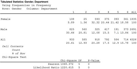
Thus, the value of chi-square statistic is 1,068.372.

It is known that under the null hypothesis $H_0$ the test statistic ${\chi }^2={\displaystyle \sum \frac{{\left(O-E\right)}^2}{E}}$ follows  chi-square distribution with $\left(r-1\right)\left(c-1\right)$ degrees of freedom for r number of rows and c number of columns, provided that all the expected frequencies are greater than or equal to 5.

In the given question there are 2 rows and 6 columns.

Hence, the degrees of freedom is

$\begin{array}{c}\left(r-1\right)\left(c-1\right)=\left(2-1\right)\left(6-1\right)\\ =\left(1\right)\left(5\right)\\ =5\end{array}$.

Thus, the degree of freedom is 5.

It is known that when the null hypothesis $H_0$ is true the chi-square statistic for a test of independence, follows approximately chi-square distribution provided that all the expected frequencies are 5 or more.

It is found that all the expected frequencies corresponding to all rows and columns of the given contingency table are more than 5.

Hence, the test of independence is appropriate.

Step 5:

Critical value:

In a test of hypotheses the critical value is the point by which one can reject or accept the null hypothesis.

Software procedure:

Step-by-step software procedure to obtain critical value using MINITAB software is as follows:

• Select Graph > Probability distribution plot > view probability
• Select Chi -Square under distribution.
• In Degrees of freedom, enter 5.
• Choose Probability Value and Right Tail for the region of the curve to shade.
• Enter the Probability value as 0.01 under shaded area.
• Select OK.
• Output using MINITAB software is given below:

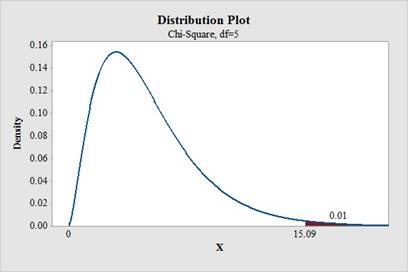
Hence, the critical value at $\alpha =0.01$ is 15.09.

  Rejection rule:

If the ${\chi }^2$ value is greater than or equal to critical value, that is ${\chi }^2\ge {\chi }_{\alpha ;k-1}^2$, then reject the null hypothesis $H_0$. Otherwise, do not reject $H_0$.

Step 6:

Conclusion:

Here, the ${\chi }^2$ value is greater than the critical value.

That is, ${\chi }^2\left(=1,068.372\right)>{\chi }_{0.01,5}^2\left(=15.09\right)$

Thus, the decision is “reject the null hypothesis”.

Thus, there is enough evidence to conclude that the gender differs among departments.