Mathematical Statistics with Applications
7th Edition
ISBN: 9781111798789
Author: Dennis O. Wackerly
Publisher: Cengage Learning
bartleby

Videos

Question
Book Icon
Chapter 10.8, Problem 77E

a.

To determine

State whether there is sufficient evidence to conclude that there is a difference in the mean verbal SAT scores for high school students intending to major in engineering and in language at the α=0.05.

Obtain the associated p-value.

a.

Expert Solution
Check Mark

Answer to Problem 77E

Yes, there is sufficient evidence to conclude that there is a difference in the mean verbal SAT scores for high school students intending to major in engineering and in language at the α=0.05.

The attained significance level is approximately 0.

Explanation of Solution

The test hypotheses are given as follows:

Denote μ1 as the mean verbal SAT scores for high school students intending to major in engineering and μ2 as the mean verbal SAT scores for high school students intending to major in language.

Null hypothesis:

H0:μ1=μ2

That is, there is no difference in the mean verbal SAT scores for high school students intending to major in engineering and in language.

Alternative hypothesis:

Ha:μ1μ2

That is, there is a difference in the mean verbal SAT scores for high school students intending to major in engineering and in language.

Assumptions:

It is assumed that Y1,Y2,...Yn is an independent random sample from a normal population with σ12=σ22.

Test statistic:

For large sample n, the sample means Y¯1andY¯2 are the point estimate of μ1 and μ2, respectively. Thus, the test statistic is as given below:

T=(Y¯1Y¯2)D0Sp1n1+1n2

Where, D0=μ1μ2  is the difference, n1and n2 are the sample size of two population, σ12andσ22 are the population variances, and Sp is the pooled estimate of σ2.

Here,

 Sp=(n11)s12+(n21)s22n1+n22.

The pooled estimate of σ2 is obtained as given below:

Substitute s1 as 42, s2 as 45, n1 as 15, and n2 as 15.

Sp=(151)(42)2+(151)(45)215+152=24,696+28,35028=1,894.5=43.53

The test statistic is obtained as given below:

Substitute Y¯1 as 446, Y¯2 as 534, D0 as 0, Sp as 43.53, n1 as 15, and n2 as 15.

T=(446534)0(43.53)115+115=8815.895=5.54

Degrees of freedom:

v=n1+n22=15+152=28

Here, the probability of the test statistic 2[P(T>5.54)] is obtained as given below:

Step-by-step procedure to obtain the critical value using Applet:

  • Go to Applets/Simulations under Book Resources.
  • Select Student’s t Probabilities and Quantiles.
  • In df, enter 28.
  • In x:, enter 5.54.

The output obtained is as follows:

Mathematical Statistics with Applications, Chapter 10.8, Problem 77E , additional homework tip  1

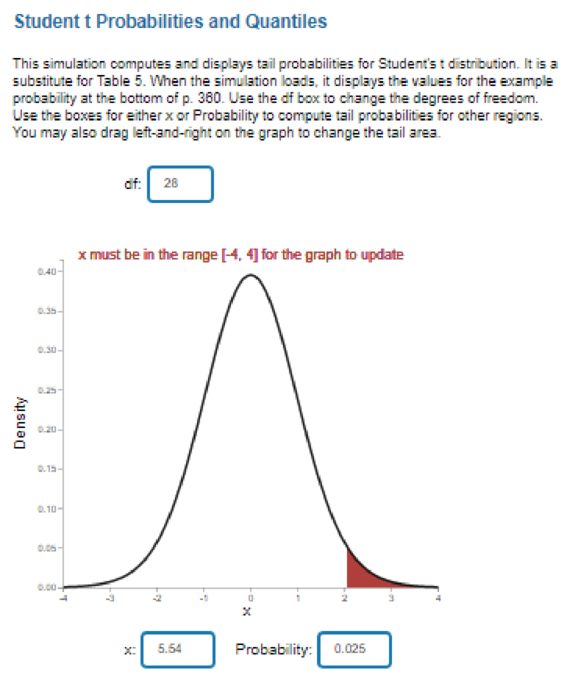
From the output, it is clear that the value must be in the range [–4,4]. Here, the value of x is out of the range. Therefore, the probability of 2[P(T>5.54)] will be approximately 0.

Decision rule:

  • If p-valueα, reject the null hypothesis.
  • Otherwise, fail to reject the null hypothesis.

Conclusion:

Here, the p-value is less than the significance level of 0.05.

Therefore, by the decision rule, reject the null hypothesis.

Therefore, the data provide the evidence to support the claim that there is a difference in the mean verbal SAT scores for high school students intending to major in engineering and in language at α=0.05.

b.

To determine

State whether the results in Part (a) are consistent with Exercise 8.90(a).

b.

Expert Solution
Check Mark

Explanation of Solution

On observing Exercise 8.90(a), the confidence interval of difference in the mean verbal SAT score for high school students intending to major in engineering and in language is (–120.55, –55.45).

Since 0 does not lie in the confidence interval, the null hypothesis is rejected and supports the conclusion that is same as in Part (a).

Therefore, the results in Part (a) are consistent with Exercise 8.90(a).

c.

To determine

State whether there is sufficient evidence to conclude that there is a difference in the mean math SAT scores for high school students intending to major in engineering and in language at the α=0.05.

Obtain the associated p-value.

c.

Expert Solution
Check Mark

Answer to Problem 77E

Yes, there is sufficient evidence to conclude that there is a difference in the mean math SAT scores for high school students intending to major in engineering and in language at the α=0.05.

The attained significance level is approximately 0.

Explanation of Solution

The test hypotheses are given as follows:

Denote μ1 as the mean math SAT scores for high school students intending to major in engineering and μ2 as the mean math SAT scores for high school students intending to major in language.

Null hypothesis:

H0:μ1=μ2

That is, there is no difference in mean math SAT scores for high school students intending to major in engineering and in language.

Alternative hypothesis:

Ha:μ1μ2

That is, there is a difference in mean math SAT scores for high school students intending to major in engineering and in language.

Assumptions:

It is assumed that Y1,Y2,...Yn is a independent random sample from a normal population with σ12=σ22.

Test statistic:

For large sample n, the sample means Y¯1andY¯2 are the point estimate of μ1 and μ2, respectively. Thus, the test statistic is as given below:

T=(Y¯1Y¯2)D0Sp1n1+1n2

Where, D0=μ1μ2  is the difference, n1and n2 are the sample sizes of two populations, σ12andσ22 are the population variances, and Sp is the pooled estimate of σ2.

Here,

 Sp=(n11)s12+(n21)s22n1+n22.

The pooled estimate of σ2 is obtained as given below:

Substitute s1 as 57, s2 as 52, n1 as 15, and n2 as 15.

Sp=(151)(57)2+(151)(52)215+152=45,486+37,85628=2,976.5=54.56

The test statistic is obtained as given below:

Substitute Y¯1 as 548, Y¯2 as 517, D0 as 0, Sp as 54.56, n1 as 15, and n2 as 15.

T=(548517)0(54.56)115+115=3119.9225=1.56

Degrees of freedom:

v=n1+n22=15+152=28

Here, the probability of test statistic 2[P(T>1.56)] is obtained as given below:

Step-by-step procedure to obtain the critical value using Applet:

  • Go to Applets/Simulations under Book Resources.
  • Select Student’s t Probabilities and Quantiles.
  • In df, enter 28.
  • In x:, enter 1.56.

The output obtained is as follows:

Mathematical Statistics with Applications, Chapter 10.8, Problem 77E , additional homework tip  2

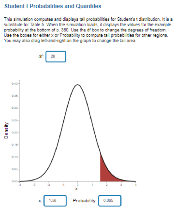
From the output, the probability of P(T>1.56) will be 0.65.

Therefore, the probability of 2P(T>1.56) is 0.13(2×0.065)_.

Conclusion:

Here, the p-value is greater than the significance level of 0.05.

Therefore, by the decision rule, fail to reject the null hypothesis.

Therefore, the data do not provide the evidence to support the claim that there is difference in mean math SAT scores for high school students intending to major in engineering and in language at α=0.05.

d.

To determine

State whether the results in Part (c) are consistent with Exercise 8.90(b).

d.

Expert Solution
Check Mark

Explanation of Solution

On observing Exercise 8.90(b), the confidence interval of difference in the mean math SAT score for high school students intending to major in engineering and in language is (-9.799, 71.799).

Since 0 lie in the confidence interval, the null hypothesis is not rejected and supports the conclusion that is same as in Part (c).

Therefore, the results in Part (c) are consistent with Exercise 8.90(b).

Want to see more full solutions like this?

Subscribe now to access step-by-step solutions to millions of textbook problems written by subject matter experts!
Students have asked these similar questions
Independent random samples of 27 people living on the west side of a city and 26 people living on the east side of a city were taken to determine if the income levels of west side residents are less than the income levels of east side residents. Given the testing statistics below, determine if the data provides sufficient evidence to conclude that the income levels of west side residents are less than the income levels of east side residents, at the 4% significance level. H0:μw≥μeHa:μw<μe t0=−2.344 t0.04=−2.107   Select the correct answer below: Yes; the test statistic is greater than the critical value. No; the test statistic is less than the critical value. No; the test statistic is greater than the critical value. Yes; the test statistic is less than the critical value.
Independent random samples of 27 people living on the west side of a city and 26 people living on the east side of a city were taken to determine if the income levels of west side residents are less than the income levels of east side residents. Given the testing statistics below, determine if the data provides sufficient evidence to conclude that the income levels of west side residents are less than the income levels of east side residents, at the 4% significance level. H0:μw≥μeHa:μw<μe t0=−2.344 t0.04=−2.107
Independent random samples of 31 people living on the west side of a city and 25 people living on the east side of a city were taken to determine if the income levels of west side residents are greater than the income levels of east side residents. Given the testing statistics below, determine if the data provides sufficient evidence to conclude that the income levels of west side residents are greater than the income levels of east side residents, at the 2% significance level. H0:μw≤μeHa:μw>μe t0=0.511 t0.02=2.104 Select the correct answer below:   Yes; the test statistic is greater than the critical value.   No; the test statistic is greater than the critical value.   No; the test statistic is less than the critical value.   Yes; the test statistic is less than the critical value.

Chapter 10 Solutions

Mathematical Statistics with Applications

Ch. 10.3 - The output voltage for an electric circuit is...Ch. 10.3 - The Rockwell hardness index for steel is...Ch. 10.3 - Shear strength measurements derived from...Ch. 10.3 - Prob. 22ECh. 10.3 - Studies of the habits of white-tailed deer...Ch. 10.3 - A study by Childrens Hospital in Boston indicates...Ch. 10.3 - An article in American Demographics reports that...Ch. 10.3 - According to the Washington Post, nearly 45% of...Ch. 10.3 - The state of California is working very hard to...Ch. 10.3 - Prob. 28ECh. 10.3 - Prob. 29ECh. 10.3 - Prob. 30ECh. 10.3 - Prob. 31ECh. 10.3 - In March 2001, a Gallup poll asked. How would you...Ch. 10.3 - A political researcher believes that the fraction...Ch. 10.3 - Exercise 8.58 stated that a random sample of 500...Ch. 10.3 - Michael Sosin investigated determinants that...Ch. 10.3 - Prob. 36ECh. 10.4 - Refer to Exercise 10.19. If the voltage falls as...Ch. 10.4 - Refer to Exercise 10.20. The steel is sufficiently...Ch. 10.4 - Refer to Exercise 10.30. Calculate the value of ...Ch. 10.4 - Refer to Exercise 10.33. The political researcher...Ch. 10.4 - Refer to Exercise 10.34. Using the rejection...Ch. 10.4 - In Exercises 10.34 and 10.41, how large should the...Ch. 10.4 - A random sample of 37 second graders who...Ch. 10.4 - Refer to Exercise 10.43. Find the sample sizes...Ch. 10.5 - Refer to Exercise 10.21. Construct a 99%...Ch. 10.5 - Prob. 46ECh. 10.5 - Prob. 47ECh. 10.5 - Prob. 48ECh. 10.5 - Prob. 49ECh. 10.6 - High airline occupancy rates on scheduled flights...Ch. 10.6 - Two sets of elementary schoolchildren were taught...Ch. 10.6 - A biologist has hypothesized that high...Ch. 10.6 - How would you like to live to be 200 years old?...Ch. 10.6 - Do you believe that an exceptionally high...Ch. 10.6 - A check-cashing service found that approximately...Ch. 10.6 - Prob. 56ECh. 10.6 - Prob. 57ECh. 10.6 - Prob. 58ECh. 10.8 - Why is the Z test usually inappropriate as a test...Ch. 10.8 - Prob. 62ECh. 10.8 - A chemical process has produced, on the average,...Ch. 10.8 - A coin-operated soft-drink machine was designed to...Ch. 10.8 - Operators of gasoline-fueled vehicles complain...Ch. 10.8 - Researchers have shown that cigarette smoking has...Ch. 10.8 - Nutritional information provided by Kentucky Fried...Ch. 10.8 - Prob. 68ECh. 10.8 - Two methods for teaching reading were applied to...Ch. 10.8 - A study was conducted by the Florida Game and Fish...Ch. 10.8 - Under normal conditions, is the average body...Ch. 10.8 - Prob. 72ECh. 10.8 - In Exercise 8.83, we presented some data collected...Ch. 10.8 - Prob. 74ECh. 10.8 - Prob. 75ECh. 10.8 - Prob. 76ECh. 10.8 - Prob. 77ECh. 10.9 - A manufacturer of hard safety hats for...Ch. 10.9 - Prob. 79ECh. 10.9 - Prob. 80ECh. 10.9 - Prob. 81ECh. 10.9 - Exercises 8.83 and 10.73 presented some data...Ch. 10.9 - Prob. 83ECh. 10.9 - An experiment published in The American Biology...Ch. 10.9 - Prob. 85ECh. 10.9 - Aptitude tests should produce scores with a large...Ch. 10.9 - Prob. 87ECh. 10.10 - Refer to Exercise 10.2. Find the power of the test...Ch. 10.10 - Prob. 89ECh. 10.10 - Refer to Exercise 10.5. a Find the power of test 2...Ch. 10.10 - Let Y1, Y2,, Y20 be a random sample of size n = 20...Ch. 10.10 - Consider the situation described in Exercise...Ch. 10.10 - For a normal distribution with mean and variance...Ch. 10.10 - Suppose that Y1, Y2, ,Yn constitute a random...Ch. 10.10 - Prob. 95ECh. 10.10 - Prob. 96ECh. 10.10 - Prob. 97ECh. 10.10 - Prob. 98ECh. 10.10 - Prob. 99ECh. 10.10 - Prob. 100ECh. 10.10 - Prob. 101ECh. 10.10 - Prob. 102ECh. 10.10 - Prob. 103ECh. 10.10 - Refer to the random sample of Exercise 10.103. a...Ch. 10.11 - Let Y1, Y2,, Yn denote a random sample from a...Ch. 10.11 - A survey of voter sentiment was conducted in four...Ch. 10.11 - Prob. 107ECh. 10.11 - Prob. 108ECh. 10.11 - Let X1, X2,, Xm denote a random sample from the...Ch. 10.11 - Show that a likelihood ratio test depends on the...Ch. 10.11 - Suppose that we are interested in testing the...Ch. 10.11 - Prob. 112ECh. 10.11 - Refer to Exercise 10.112. Show that in testing of...Ch. 10.11 - Prob. 114ECh. 10 - True or False. a If the p-value for a test is...Ch. 10 - Prob. 116SECh. 10 - Prob. 117SECh. 10 - Prob. 118SECh. 10 - Prob. 119SECh. 10 - Prob. 120SECh. 10 - Prob. 121SECh. 10 - Prob. 122SECh. 10 - A pharmaceutical manufacturer purchases a...Ch. 10 - Prob. 124SECh. 10 - Prob. 125SECh. 10 - Prob. 126SECh. 10 - Prob. 127SECh. 10 - Prob. 128SECh. 10 - Prob. 129SECh. 10 - Prob. 130SE
Knowledge Booster
Background pattern image
Statistics
Learn more about
Need a deep-dive on the concept behind this application? Look no further. Learn more about this topic, statistics and related others by exploring similar questions and additional content below.
Similar questions
Recommended textbooks for you
Text book image
Glencoe Algebra 1, Student Edition, 9780079039897...
Algebra
ISBN:9780079039897
Author:Carter
Publisher:McGraw Hill
Hypothesis Testing using Confidence Interval Approach; Author: BUM2413 Applied Statistics UMP;https://www.youtube.com/watch?v=Hq1l3e9pLyY;License: Standard YouTube License, CC-BY
Hypothesis Testing - Difference of Two Means - Student's -Distribution & Normal Distribution; Author: The Organic Chemistry Tutor;https://www.youtube.com/watch?v=UcZwyzwWU7o;License: Standard Youtube License