
To use a software to create Normal quantile plots for each of the three groups of the forest plots and explain are the three distributions roughly Normal and what are the most prominent deviations from Normality that you see.
Answer to Problem 11.51E
Yes, the three groups are roughly Normal.
Explanation of Solution
In the question, the data is given that described of the effects of logging on counts in the Borneo rainforest as:
Thus, we will use the excel to construct the Normal quantile plot by using z-scores. And the excel
So, for group one, we have the following calculation as:
| Group 1 | Rank | Rank proportion | Rank based z score | Group 1 |
| 16 | 1 | =(AA81-0.5)/COUNT($Z$81:$Z$92) | =NORMSINV(AB81) | 16 |
| 19 | 2 | =(AA82-0.5)/COUNT($Z$81:$Z$92) | =NORMSINV(AB82) | 19 |
| 19 | 3 | =(AA83-0.5)/COUNT($Z$81:$Z$92) | =NORMSINV(AB83) | 19 |
| 20 | 4 | =(AA84-0.5)/COUNT($Z$81:$Z$92) | =NORMSINV(AB84) | 20 |
| 21 | 5 | =(AA85-0.5)/COUNT($Z$81:$Z$92) | =NORMSINV(AB85) | 21 |
| 22 | 6 | =(AA86-0.5)/COUNT($Z$81:$Z$92) | =NORMSINV(AB86) | 22 |
| 24 | 7 | =(AA87-0.5)/COUNT($Z$81:$Z$92) | =NORMSINV(AB87) | 24 |
| 27 | 8 | =(AA88-0.5)/COUNT($Z$81:$Z$92) | =NORMSINV(AB88) | 27 |
| 27 | 9 | =(AA89-0.5)/COUNT($Z$81:$Z$92) | =NORMSINV(AB89) | 27 |
| 28 | 10 | =(AA90-0.5)/COUNT($Z$81:$Z$92) | =NORMSINV(AB90) | 28 |
| 29 | 11 | =(AA91-0.5)/COUNT($Z$81:$Z$92) | =NORMSINV(AB91) | 29 |
| 33 | 12 | =(AA92-0.5)/COUNT($Z$81:$Z$92) | =NORMSINV(AB92) | 33 |
The result is as:
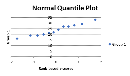
| Group 1 | Rank | Rank proportion | Rank based z score | Group 1 |
| 16 | 1 | 0.041667 | -1.73166 | 16 |
| 19 | 2 | 0.125 | -1.15035 | 19 |
| 19 | 3 | 0.208333 | -0.81222 | 19 |
| 20 | 4 | 0.291667 | -0.54852 | 20 |
| 21 | 5 | 0.375 | -0.31864 | 21 |
| 22 | 6 | 0.458333 | -0.10463 | 22 |
| 24 | 7 | 0.541667 | 0.104633 | 24 |
| 27 | 8 | 0.625 | 0.318639 | 27 |
| 27 | 9 | 0.708333 | 0.548522 | 27 |
| 28 | 10 | 0.791667 | 0.812218 | 28 |
| 29 | 11 | 0.875 | 1.150349 | 29 |
| 33 | 12 | 0.958333 | 1.731664 | 33 |
Thus, we will select the last two column and then go to the insert tab and select the chart option and then select the plot, so the normal quantile plot is as:
So, for the group two we have the calculation as:
| Group 2 | Rank | Rank proportion | Rank based z score | Group 2 |
| 2 | 1 | =(AG81-0.5)/COUNT($AF$81:$AF$92) | =NORMSINV(AH81) | 2 |
| 9 | 2 | =(AG82-0.5)/COUNT($AF$81:$AF$92) | =NORMSINV(AH82) | 9 |
| 12 | 3 | =(AG83-0.5)/COUNT($AF$81:$AF$92) | =NORMSINV(AH83) | 12 |
| 12 | 4 | =(AG84-0.5)/COUNT($AF$81:$AF$92) | =NORMSINV(AH84) | 12 |
| 14 | 5 | =(AG85-0.5)/COUNT($AF$81:$AF$92) | =NORMSINV(AH85) | 14 |
| 14 | 6 | =(AG86-0.5)/COUNT($AF$81:$AF$92) | =NORMSINV(AH86) | 14 |
| 15 | 7 | =(AG87-0.5)/COUNT($AF$81:$AF$92) | =NORMSINV(AH87) | 15 |
| 17 | 8 | =(AG88-0.5)/COUNT($AF$81:$AF$92) | =NORMSINV(AH88) | 17 |
| 17 | 9 | =(AG89-0.5)/COUNT($AF$81:$AF$92) | =NORMSINV(AH89) | 17 |
| 18 | 10 | =(AG90-0.5)/COUNT($AF$81:$AF$92) | =NORMSINV(AH90) | 18 |
| 19 | 11 | =(AG91-0.5)/COUNT($AF$81:$AF$92) | =NORMSINV(AH91) | 19 |
| 20 | 12 | =(AG92-0.5)/COUNT($AF$81:$AF$92) | =NORMSINV(AH92) | 20 |
Thus, the result is as:
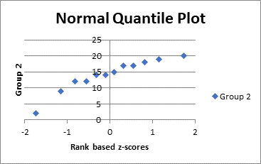
| Group 2 | Rank | Rank proportion | Rank based z score | Group 2 |
| 2 | 1 | 0.0416667 | -1.731664396 | 2 |
| 9 | 2 | 0.125 | -1.15034938 | 9 |
| 12 | 3 | 0.2083333 | -0.812217801 | 12 |
| 12 | 4 | 0.2916667 | -0.548522283 | 12 |
| 14 | 5 | 0.375 | -0.318639364 | 14 |
| 14 | 6 | 0.4583333 | -0.104633456 | 14 |
| 15 | 7 | 0.5416667 | 0.104633456 | 15 |
| 17 | 8 | 0.625 | 0.318639364 | 17 |
| 17 | 9 | 0.7083333 | 0.548522283 | 17 |
| 18 | 10 | 0.7916667 | 0.812217801 | 18 |
| 19 | 11 | 0.875 | 1.15034938 | 19 |
| 20 | 12 | 0.9583333 | 1.731664396 | 20 |
Thus, we will select the last two column and then go to the insert tab and select the chart option and then select the plot, so the normal quantile plot is as:
So, for the group three we have the calculation as:
| Group3 | Rank | Rank proportion | Rank based z score | Group3 |
| 4 | 1 | =(T81-0.5)/COUNT($S$81:$S$89) | =NORMSINV(U81) | 4 |
| 12 | 2 | =(T82-0.5)/COUNT($S$81:$S$89) | =NORMSINV(U82) | 12 |
| 12 | 3 | =(T83-0.5)/COUNT($S$81:$S$89) | =NORMSINV(U83) | 12 |
| 15 | 4 | =(T84-0.5)/COUNT($S$81:$S$89) | =NORMSINV(U84) | 15 |
| 18 | 5 | =(T85-0.5)/COUNT($S$81:$S$89) | =NORMSINV(U85) | 18 |
| 18 | 6 | =(T86-0.5)/COUNT($S$81:$S$89) | =NORMSINV(U86) | 18 |
| 19 | 7 | =(T87-0.5)/COUNT($S$81:$S$89) | =NORMSINV(U87) | 19 |
| 22 | 8 | =(T88-0.5)/COUNT($S$81:$S$89) | =NORMSINV(U88) | 22 |
| 22 | 9 | =(T89-0.5)/COUNT($S$81:$S$89) | =NORMSINV(U89) | 22 |
The result is as:
| Group3 | Rank | Rank proportion | Rank based z score | Group3 |
| 4 | 1 | 0.055555556 | -1.593218818 | 4 |
| 12 | 2 | 0.166666667 | -0.967421566 | 12 |
| 12 | 3 | 0.277777778 | -0.589455798 | 12 |
| 15 | 4 | 0.388888889 | -0.282216147 | 15 |
| 18 | 5 | 0.5 | 0 | 18 |
| 18 | 6 | 0.611111111 | 0.282216147 | 18 |
| 19 | 7 | 0.722222222 | 0.589455798 | 19 |
| 22 | 8 | 0.833333333 | 0.967421566 | 22 |
| 22 | 9 | 0.944444444 | 1.593218818 | 22 |
Thus, we will select the last two column and then go to the insert tab and select the chart option and then select the plot, so the normal quantile plot is as:
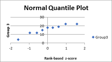
Thus, we can see that in the three groups the points are approximately in a straight line and increasing in nature. Thus, we can say that the three groups are approximately follows
Want to see more full solutions like this?
Chapter 11 Solutions
Practice of Statistics in the Life Sciences

 MATLAB: An Introduction with ApplicationsStatisticsISBN:9781119256830Author:Amos GilatPublisher:John Wiley & Sons Inc
 Probability and Statistics for Engineering and th...StatisticsISBN:9781305251809Author:Jay L. DevorePublisher:Cengage Learning
 Statistics for The Behavioral Sciences (MindTap C...StatisticsISBN:9781305504912Author:Frederick J Gravetter, Larry B. WallnauPublisher:Cengage Learning
 Elementary Statistics: Picturing the World (7th E...StatisticsISBN:9780134683416Author:Ron Larson, Betsy FarberPublisher:PEARSON
 The Basic Practice of StatisticsStatisticsISBN:9781319042578Author:David S. Moore, William I. Notz, Michael A. FlignerPublisher:W. H. Freeman
 Introduction to the Practice of StatisticsStatisticsISBN:9781319013387Author:David S. Moore, George P. McCabe, Bruce A. CraigPublisher:W. H. Freeman