
Concept explainers
Videos
(a)
To find: The multiple regression for BMI using
(a)
Answer to Problem 25E
Solution: The required multiple regression model is
Explanation of Solution
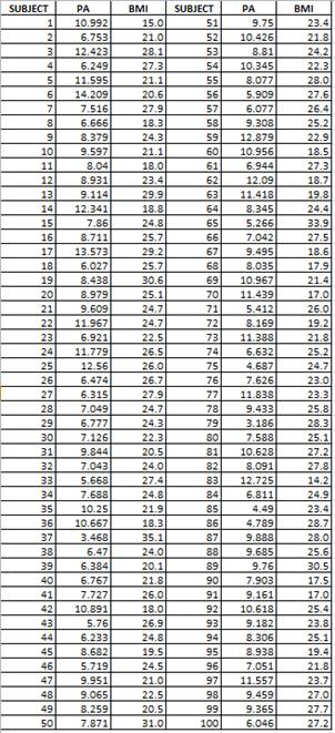
Given: The data for the PA and BMI are given below:
Calculation: The explanatory variables are
To obtain multiple
Step 1: Enter the data in Minitab worksheet.
Step 2: Go to Calc>Calculator.
Step 3: Enter
Step 4: Click OK.
Step 5: Repeat the steps. Enter
Step 6: Go to Stat > Regression > Regression
Step 7: Select BMI in Response and select
Step 8: Click OK.
The multiple regression model is obtained as
(b)
To find: The value of
(b)
Answer to Problem 25E
Solution: The value of
Explanation of Solution
(c)
To graph: The Normal quantile plot.
(c)
Explanation of Solution
Graph: To perform the multiple regression by using year and census count as explanatory variables use Minitab. Follow the steps below:
Step 1: Enter the data in Minitab worksheet.
Step 2: Go to Stat> Regression >Regression.
Step 3: Select BMI in Response and select
Step 4: Click on Graphs and select “Residuals versus fits.”
Step 5: Click OK.
The residual plot is obtained as:
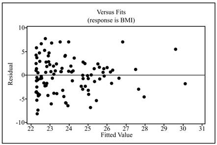
Interpretation: From the obtained residual plot, it can be concluded that the plot represents no pattern and the data points are randomly scattered.
(d)
To test: The hypothesis that coefficient of the variable
(d)
Answer to Problem 25E
Solution: There is enough evidence to conclude that there is no linear increase over time.
Explanation of Solution
Calculation: From the output which is obtained in part (b), the regression equation is
The level of significance is 0.05. The test statistic under null hypothesis is calculated as:
The p-value can be calculated as:
The p-value is 0.0678.
Conclusion: The obtained p-value is greater than the significance level. Hence, there is enough evidence to conclude that the quadratic term contributes insignificantly to the fit.
Want to see more full solutions like this?
Chapter 11 Solutions
Introduction to the Practice of Statistics


 MATLAB: An Introduction with ApplicationsStatisticsISBN:9781119256830Author:Amos GilatPublisher:John Wiley & Sons Inc
 Probability and Statistics for Engineering and th...StatisticsISBN:9781305251809Author:Jay L. DevorePublisher:Cengage Learning
 Statistics for The Behavioral Sciences (MindTap C...StatisticsISBN:9781305504912Author:Frederick J Gravetter, Larry B. WallnauPublisher:Cengage Learning
 Elementary Statistics: Picturing the World (7th E...StatisticsISBN:9780134683416Author:Ron Larson, Betsy FarberPublisher:PEARSON
 The Basic Practice of StatisticsStatisticsISBN:9781319042578Author:David S. Moore, William I. Notz, Michael A. FlignerPublisher:W. H. Freeman
 Introduction to the Practice of StatisticsStatisticsISBN:9781319013387Author:David S. Moore, George P. McCabe, Bruce A. CraigPublisher:W. H. Freeman